
back to the start of the tutorial
The fourth step of this tutorial is the global analysis of the DNA and Protein mixture using data from the remaining cells of the AUC run. (Please refer to the Experimental Details to see the loading concentrations of the different cells)
We will use data obtained from the individual analysis of the DNA and the protein as fixed parameters in the analysis of the mixture to save fitting time.
For the DNA, the apparent mass of 23.9 kDa will be the value we use, in conjunction with the v-bar value of the protein of 0.743. (Again, the true molar mass is different, and so is the v-bar, but the buoyant molar mass determined by the product M*(1-vbar*rho) is correct (this is the important quantity), and by doing it this way we can work with the same apparent vbar for the protein and the DNA.) The extinction coefficients are 449100 OD/Mcm at 260 nm (this was fixed to the theoretical value), 186,400 OD/Mcm at 230 nm, and 269,600 OD/Mcm at 280 nm. These values will also be used as fixed prior knowledge for the multi-wavelength analysis of the mixture of DNA with protein.
For the protein, the Mw value is 9.3 kDa. This is within the usual range of precision, and we will accept the value of 9.3 kDa (and use it in the analysis of the mixture), continuing to use 0.743 ml/g as our vbar scale. The extinction coefficient are 4868 OD/Mcm at 260 nm, and 8480 OD/Mcm at 280 nm (the latter was fixed to the theoretical value). These values will also be used as fixed prior knowledge for the multi-wavelength analysis of the mixture of DNA with protein.
Based on the protein analysis, we have decided to use only 2 wavelengths, 280 and 260 nm.
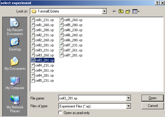
Step 12: Selecting the .xp files from Cells 3-7 and opening them in Sedphat.
We also have already used Sedfit to prepare the SE raw data files and generate the xp-files for all cells. We don't need to redo this. Therefore, we jump directly to the next step, loading the data from the mixture of DNA and the protein into a new Sedphat window. Begin loading files in the same manner as before. Use the function Data->Load Experiment

, and find and load the .xp files from cells 3 through 7 at 280 and 260 nm. Remember they will be lined up in the Sedphat window in the order that they are loaded, and they will be referred to according to their number, therefore it's useful to load them systematically. In this tutorial, we choose the sequence: cell 3 at 280, cell 3 at 260, cell 4 at 280, cell 4 at 260, etc.
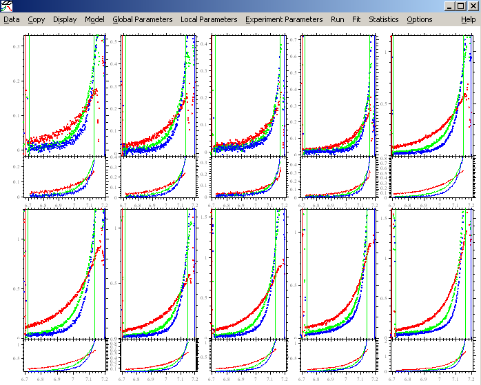
After loading all the .xp files, we end up with 10 experiments.
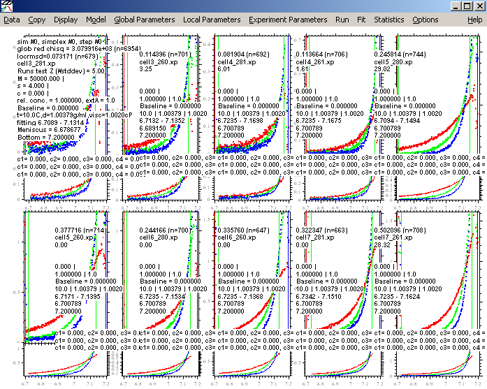
With the function "Show last fit info again", the information about each experiment will appear. Notice that the .xp file names are listed on the 4th line from the top. (The other information is not meaningful at this point.) Now, before parameters are entered, is a good time to make sure that the experiments are in the order that you want them to be.
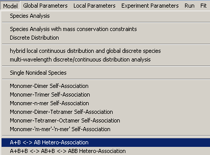
We are going to start with a Hetero-Association, single site model (A+B). Generally, for a mixture, it is a good idea to begin with this model. Even though, we do have evidence that the two site model (A+B+B) would be the correct model, we will begin here with the single-site model, in order to demonstrate why this model is not as good as the two-site model. This will give us more confidence for using the two-site model later.
Open the global parameters window.
![]()
It will open with default parameters.
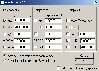
Considering "A" component to be DNA and "B" component as Protein, we will leave most of these default parameters in place at this point, but will enter the MW of A and B, fit with Mass Conservation and set the Log(Ka) value for binding constant to a good initial estimate. Association constants are in Log(10) of molar units, so to get into a range where the fitting algorithm will be able to optimize it, we will take into account our concentration range of microM (10-6 ) and enter 6 here. sA, sB and sAB are sedimentation coefficients and are insignificant here. The concentrations (atot and btot) and extinction coefficients will be entered for each experiment when the experiment parameters are entered. Incompetent fractions of A and B (incfA and incfB) will be left alone initially. In the end, our window should look like this now:
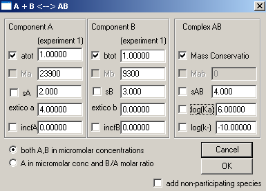
After hitting Ok, this window appears
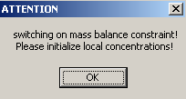
...hit Ok.
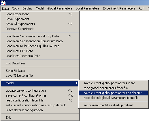
A note with regard to the default parameters. If you work with the same molecules and repeatedly use a particular model, you can set your own parameters and then go to Data-> Model-> "save current parameters as default" and have your parameters in place each time you open that particular model.
Next, set up the local parameters.
![]()
This can get very complicated, so make sure you have the correct concentrations available for reference.
Begin with exp # 1. This is AUC cell #3 scanned at 280.
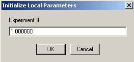
Concentration A of exp #1 is DNA at 0.3uM. Link it to exp #1 (this means there is no redirection (or link) of this parameter).
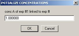
Enter the concentration of DNA, component A (ca),

Then to component B, the protein. It is also not redirected, i.e. linked to itself.

Enter the concentration of protein, component B (cb), in the next window.
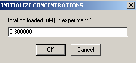
Experiment #2 is the same cell, only scanned at wave length 260,

so we can link the concentration of A to exp #1,

and the same is true for B: link it to exp #1. Hit OK.

On to exp #3.
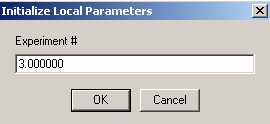
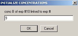
Link the DNA concentration to exp #3
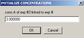
Enter the DNA concentration of experiment # 3.
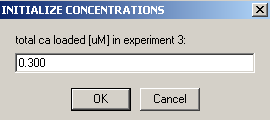
(Actually, since the concentration is the same as in xp1 (cell 1), it could have been linked, but this was not done for consistency with the following screenshots.)
Also, link the protein concentration to exp #3.
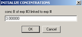
Then, enter the concentration of B in exp #3.
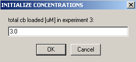
Next:
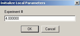
Experiment #4 is cell4 at a 260 wavelength so we can link conc.A , to exp #3
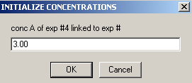
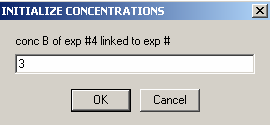
and conc. B to exp #3.
Exp #5 is cell5 at 280.

We aren't able to link the DNA concentration to any of the previous experiments.

Enter the DNA concentration here as 1.0
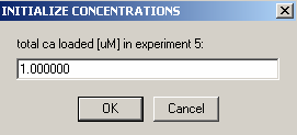
We also are not able to link the protein concentration to a previous experiment, so hit Ok here.
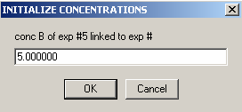
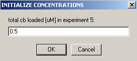
The protein concentration of cell5 is 0.5
Exp #6 is cell 5 scanned at 260 wavelength so all concentrations can be linked to exp #5.

First the DNA
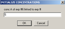
Then the protein.

On to Exp #7
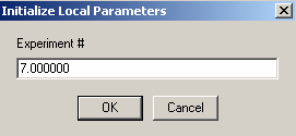
This is our cell 6, where the DNA concentration is the same as in Cell5, so link it to exp #5
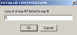
The concentration of protein is not the same so it can't be linked.
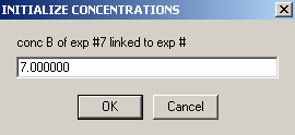
Enter the concentration of protein in cell6 here.
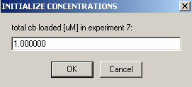
Exp #8 is cell6 at 260 wavelength so:

link conc.A to exp #5

and link conc.B to exp #7
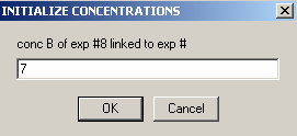
Exp #9 is cell7

The DNA concentration is the same as in exp #5, so they can be linked
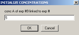
the protein concentration is not linked to any other experiments.

Enter protein concentration
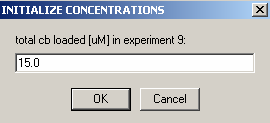
Exp #10 is cell7 at 260 wavelength so,
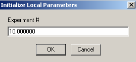
link the DNA concentration to exp #5
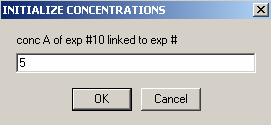
and link the protein concentration to exp #9
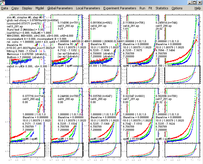
If we "display fit info again" the concentrations will now be displayed along with the Exp# of the links in the last line of each experiment's window. Take the time now to make sure all is in order.
For the current experiment, we have no indication that mass conservation is violated. We would have noticed that when analyzing the protein and the DNA by itself, we would not have been able to get a good fit with mass conservation. Therefore, we can expect that it will be conserved as well in the mixture. This may not necessarily always be the case, for example, some protein may slowly precipitate or form a surface film at the bottom of the cell, slowly depleting the mass suspended in the solution column. In this case, mass conservation would not be valid. [Notice that the mass conservation only assumes that the material that was soluble at the time of the first equilibrium will still be soluble at the time of the last equilibrium, but it does not require the absence of some initial loss, for example, adsorption to the window etc.]
But even if mass is not conserved, it is a good idea to use the Mass conservation function in the global parameters. This will eliminate the reference concentration for each component and each equilibrium scan, and therefore considerably simplify setting up the global analysis and fitting it. If you don't use mass conservation, you have to provide initial estimates for the concentration of A and B at the bottom of the cell for each rotor speed. An example of that is in the 5 windows below as the local parameters are set up for exp # 1. [Don't do that yourself when you're following the tutorial...]


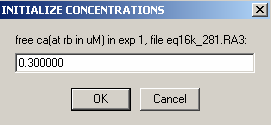
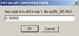
Clearly, this would be very cumbersome [and difficult to estimate since the concentration at the bottom of the cell is usually much different from the initial loading concentration]. If you need to fit without mass conservation, you can use an initial fit with mass conservation (and floating the bottom of the cell). After this has converged, switch mass conservation off, and you'll find that concentrations at the bottom of the cell have automatically been calculated based on your first fit, and you won't need to initialize them.
Back to our analysis.
Now, begin setting up the experiment parameters
![]()
Exp #1 window appears.
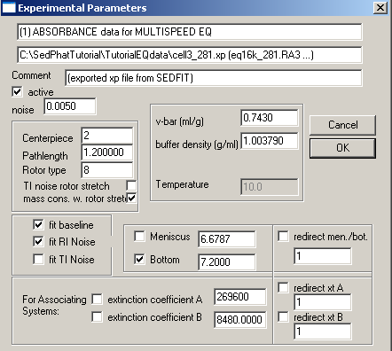
Common parameters for all 10 experiments will be the v-bar of the protein, 0.7439, the buffer density, 1.003790, fitting for RI noise and mass conservation with rotor stretching. Here in exp# 1, we will fit for the bottom and enter the extinction coefficients for this wavelength (listed on line 2 of this window), values we determined from the single component analysis of DNA and protein. In theory, we could link the extinction coefficients throughout all of these experiments and fit for them, but if we enter them for each experiment and keep them fixed, it will be one less parameter we have to fit for, since we have determined them already. Also, these values are easier to fit for in the simplex fitting of the single component analysis. Note that we're making the approximation here that there's no hyper- or hypo-chromicity at the wavelengths used. [If that would be a bad assumption in the present case, one might be able to do an experiment with dual-signal analysis combining interference data with an absorption wavelength where the spectrum does not change.]
More about the baseline options will follow below.
Hit Ok and the following 2 windows appear, asking for limits of the variation of the bottom parameter. I would usually accept the default range (although this could be refined partially, through visual inspection of the scans).
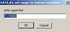
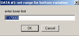
Hit Ok for both, then the experiment #2 window appears.
In exp #2, redirect the bottom to exp # 1, since it is the same cell, only a different wavelength. Enter the extinction coefficients for this wavelength and keep them fixed. Check other parameters so they match with exp#1. You may notice, after you redirect the bottom (after closing and opening this box again), the meniscus also becomes redirected even though we fixed the meniscus in the previous experiment - this is OK, since it is the same cell, and should also have the same meniscus value. With mass conservation, we are mostly concerned with where the protein ends up as it sediments away from the meniscus and lands at the bottom of the solution column. The meniscus position becomes insignificant and slight changes are tolerated. Therefore, the meniscus position does not need to be fitted for (in contrast to sedimentation velocity data, the meniscus position is frequently ill-defined by the data within our analysis range). Again, the meniscus is redirected, but it will not be fitted, since the value in experiment 1 was fixed.

Exp #3 begins cell4. Fit for the bottom, enter and fix the extinction coefficients for this wavelength,

Accept the limit here
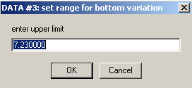
and here
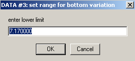
then start with exp #4
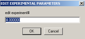
Meniscus and bottom can be redirected to exp #3 (same cell, but wavelength is 260 nm). Enter extinction coefficients for the wave length here and keep them fixed.
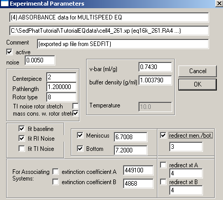
Exp #5 is cell5. Fit for the bottom, enter and fix the extinction coefficients for this wavelength,
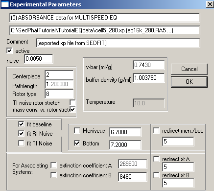
Again, redirect meniscus and bottom in exp #6 to exp #5, but don't forget to enter and fix the extinctions coefficients.
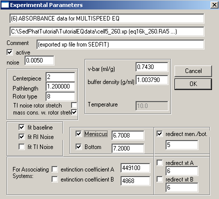
Exp #7 is cell6. Again, fit for the bottom, enter and fix the extinction coefficients.

Exp #8 is also cell6 but at wavelength 260 nm, so redirect bottom and meniscus to exp #6 and enter extinction coefficients.
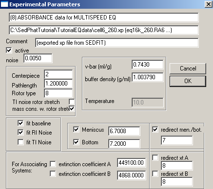
Exp #9 is the last cell in the AUC experiment, cell7. Fit for the bottom, enter and fix the extinction coefficients for this wavelength.
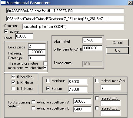
Exp #10 is the same cell as exp #9. Redirect bottom and meniscus, enter and fix extinction coefficients.
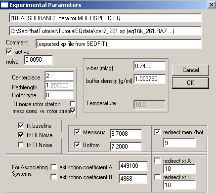
Now that all the experiment parameters are entered, display the latest information and take a few minutes to check the parameters and the links.
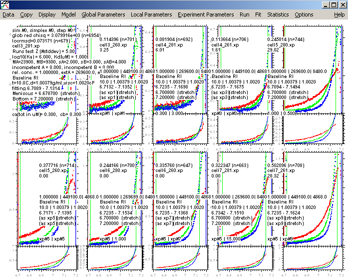
If all is in order, save the experiments.
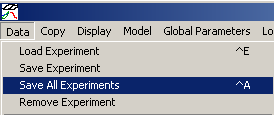
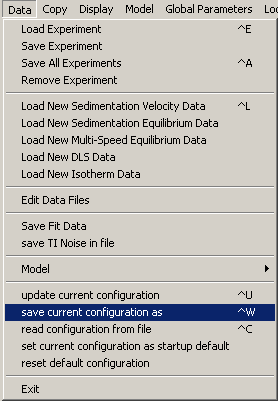
And, save this configuration
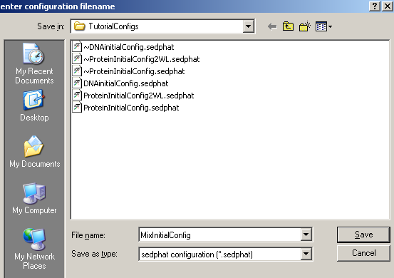
Find the correct directory and name it.
Answer "yes" to this questions.

Now, notice the name in the title heading.
![]()
Step 15: Run and Fit the Single-Site Model
Now that everything is in place, lets see how this one site model fits the data.
Begin with a global run:

The purpose of this is to check that our initial estimates for all parameters have been reasonable. Run results in the following picture:
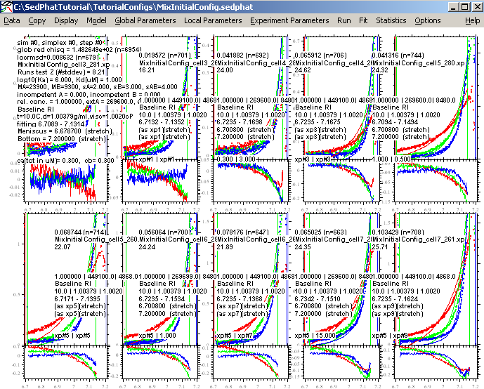
Obviously, this is a lousy match of the data, but it appears close enough for the fitting routine to optimize. Switch the fitting routine to Simplex by making sure the "Marquardt-Levenbert" is not checked.

Now execute the Global Fit

This results in (the simplex algorithm is based on an initial seeding using a random number generator, so your results may look slightly different, perhaps in the 4th or 5th decimal place).:
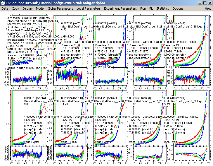
On closer inspection now, it appears that some of the fitting limits are not optimally set. (For example, look at exp 3, 9, and 10.) Lets bring in the bottom fitting limits a bit and repeat the fit. (Initially one can adjust the limits, even before doing any fits, such that the data do not exceed 1.5 OD. Having done a fit enables us sometimes to see a bit better where the data run into the region of optical artifacts close to the bottom, and should be discarded for that reason, even though they may have OD values smaller than 1.5OD.)
Do a fit again. The following looks better:
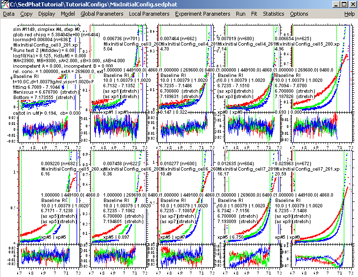
Next, turn on the Marquardt-Levenberg fit option

and fit again. Switching to Marquardt-Levenberg helps to make sure that we are really in an optimum for the fit.
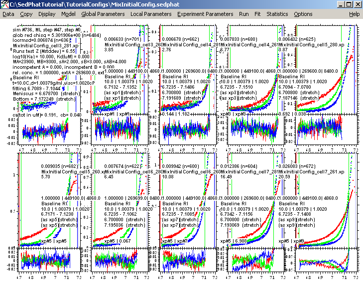
This fit is a good as we can make it with this model, but notice that the concentrations of the components are way off....sometimes even at 0.038. This is an indication that this model is possibly not ideal for this interaction. Also, notice that the for experiment 9 and 10, where we used the highest protein concentration in cell 7, the residuals are really poor. So, we are going to change to a 2 site model A+B+B, but before we switch we want to save the results of this fit, anyway. This will help us later to compare the two models.
In order not to overwrite our previous configuration "Mix Initial Configuration" which contained our initial estimates for the loading concentrations, we will save it under a new name:
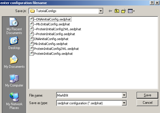
Always check yes when asked this question.

(this will keep the experimental parameters that belong to this configuration.).
Step 16: Run and Fit the Two-Site Model
When we set up an alternative model for the analysis which we'll end up comparing with the first analysis, we should make sure that we are really looking at the same data, with the same fitting limits.
If you have decided to adjust the fitting limits during the optimization of the first model, as we did here, then you need to keep these fitting limits. In this case, the new model will start from where we left off, but you will need to re-initialize the loading concentrations. Use the function
![]()
and follow the sequence outlined above in Step 13 to enter the loading concentrations.
Alternatively, if you did set up initially the fitting limits satisfactorily and didn't change it after saving the initial configuration, then you can simply open the initial configuration:
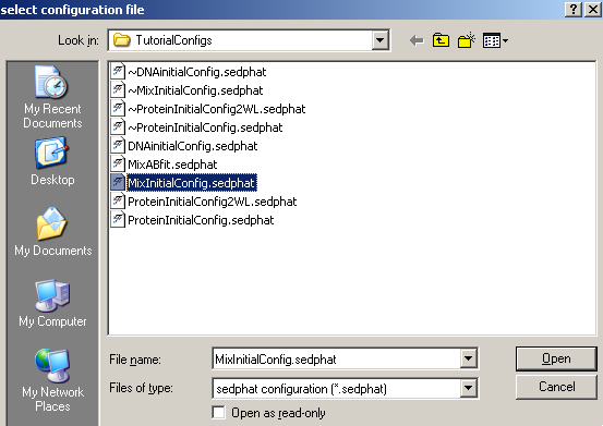
This brings up this model window. Hit Ok here.
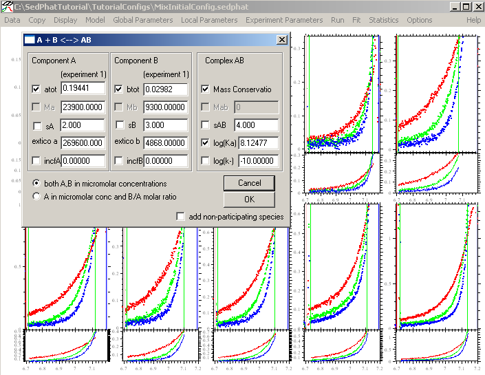
In either case, after establishing the fitting limits for fair comparison with the previous model, as well as backing up to the initial loading concentration estimates, we proceed by changing the model to two binding sites
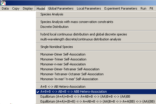
Notice that when you change models, the title heading becomes blank.
![]()
Open the global parameters window.
Make sure to enter the correct molar mass values. For the two binding constants, we will start with the assumption that both sites are equivalent. With this in mind, we enter for the first site "6" indicating a Kd in the micromolar range, and will float this value. For the second site, we leave the value log10(Ka2/Ka1) as it is...fixed at -0.6. In this way we will constraint the 2nd site to a macroscopic binding property of 1:4 with the first site, which is correct if the second site is microscopically equivalent to the first. This may not be perfect, but it is the most parsimonious assumption in the absence of any other knowledge. We can try to refine this later. Don't forget to check Mass Conservation.
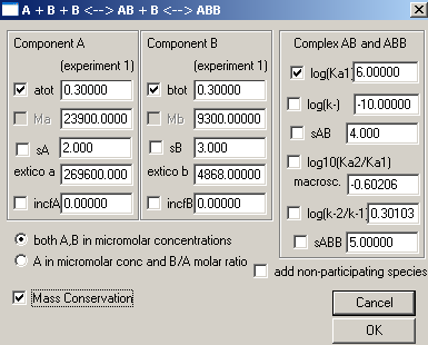
This window comes up. Just hit Ok.

One way to check that the local and experiment parameters are still in place is to "display the last fit info" as below. Another way is to just open each window and double-check. Everything looks okay.
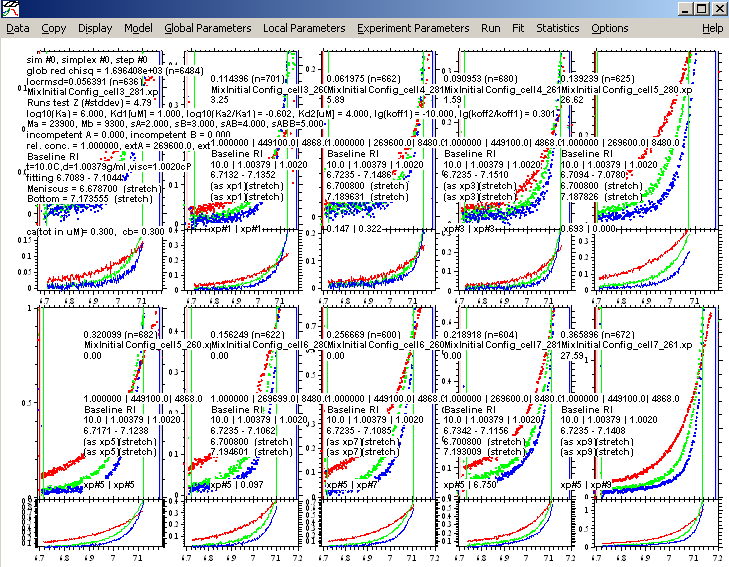
Lets do a global run

to verify that the starting estimates are reasonable (which they are). This will be followed by a global fit.

Below is the fit for 2 equivalent sites. Notice the change in ChiSq from the previous fit ( from 5.301906 to 3.152908) and the residuals at the higher concentration, where we would see the biggest difference, are much better. Also, the best-fit values of the concentrations are getting closer to what we think we've loaded. Therefore, we will accept this model as better, and save this configuration as a fair comparison to the A+B model to support our decision to change to a 2 site model.
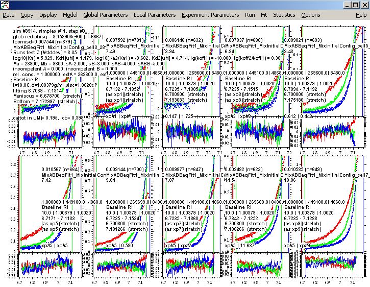
Lets save this best fit as a new configuration "MixABBeqFit1" (as described above).
We can improve the fit somewhat be switching to the Marquardt-Levenberg optimization. Also, we can readjust the fitting limits slightly, in order to eliminate data that may look suspicious. [We already made the decision that the two-site model was the correct one. For further refinement, we can justify truncating the data slightly for the further refinement and error analysis, as a conservative approach not to include data that are possibly affected by optical artifacts from too steep gradients or too radii too close to the bottom of the cell. Obviously, you don't want to exclude good data, and not exlcude reliable data that simply does not fit to the present model very well - this is a difficult judgment you have to determine for your given data.]
We end up with the following best fit of 2 equivalent binding sites.
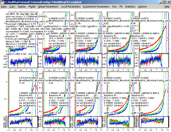
and save it as MixABBeqFit2, for further reference and comparison.
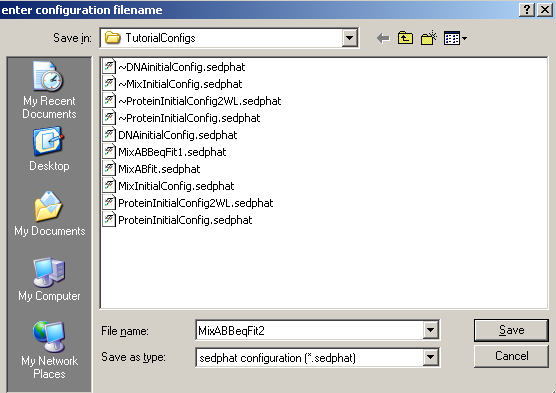
including the new corresponding xp-files.

Step 17: Two-Site Model with non-equivalent or cooperative sites
To change this same model to 2 non-equivalent binding sites, we simply let the association constant for the second site float, by floating the parameter log10(Ka2/Ka1). In doing this, the second binding site is no longer constrained to the 1:4 binding ratio and is left to find its own value. We could begin with our "MixInitialConfig" configuration, but it is more efficient to begin from where we left off with the model for two equivalent sites, since the parameters are expected to be already close.
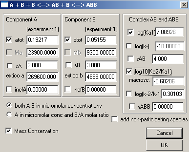
A global run produces these results:
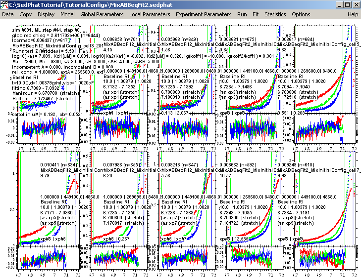
Then, finally, fitting with the ML fitting option on produces this fit below:
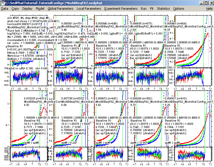
This is the best fit so far, lets save it:
We find that the chi-square of the fit from the previous equivalent site model is higher by 0.14 (always make fair comparison, i.e. same fitting limits, same constraints, and same baseline options). Is this significant? To assess this, use the function "Statistics->Critical chi-square for error surface projection". If the difference in chi-square is larger than the value displayed, we have a statistically distinguishably better (or worse) fit.
What we cannot decide from the data, however, is if the sites are equivalent and exhibit positive cooperativity, which would lead to Ka = 10^(7.993) for each site, with positive cooperativity estimated by the macroscopic enhancement factor of 10^(-0.473) = 0.34 divided by the statistical factor of 0.25, leading to 1.34fold enhancement, i.e. the macroscopic Ka2 = 10^(7.52). Alternatively, we may have two distinguishable sites, for which binding constants Ka1* and Ka2* can calculate from Ka1 and Ka2 as indicated on the SEDPHAT website.
Step 18: Making different baseline assumptions
So far, we have chosen for all experiment to fit the data with RI noise, i.e. a baseline that is radially constant, but may change for each rotor speed. There are instrumental imperfections that may require you to use this option. However, frequently, a simple baseline ('fit baseline' only) will do. Further, sometimes you may need to use the 'fit TI noise' option, as well, which assumes that there as a radial-dependent baseline profile. The latter is good, in particular, when dealing with interference optical data [and very effective in the global analysis with absorbance data, as described in Anal Biochem 326 (2004) 234-256]. You may want to do different analyses exploring the different options.
It can be a good idea to do the analysis with alternate baseline options, in order to verify that our conclusion of which is the right model, and the value of the best-fit parameters does not depend on the particular baseline treatment.
For example, we can turn on the radially-dependent baseline option (Ti noise) for each experiment:
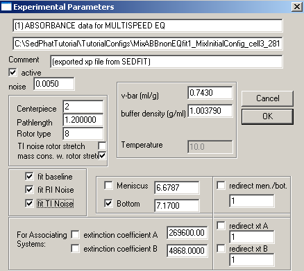
In the present case, this results in:
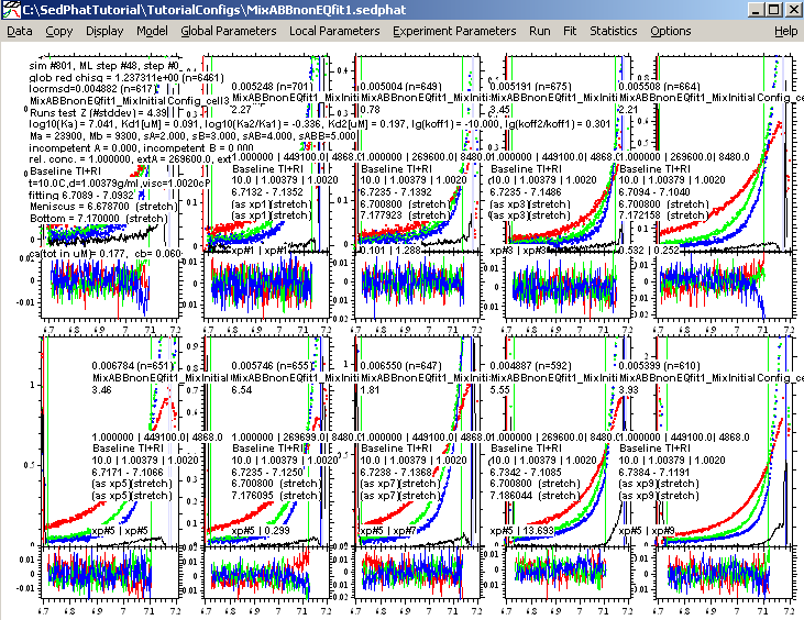
Obviously, the fit is much better, since all the blips in the data produced by tiny scratches in the window are eliminated. As described in more detail in Anal Biochem 326 (2004) 234-256, we should make sure that the calculated TI noise (the black lines) are not systematically sloping, which would be unrealistic, and indicate compensation of an imperfect model. Also, we should make sure that the TI noise option does not introduce much flexibility in the parameter estimates, which can be done by inspecting the results of the covariance matrix (Statistics->Covariance Matrix).
Step 19: On the Statistical Error Analysis
If we are convinced we have the correct model, and whish to extract error estimates, for example, for the binding constants, there are three different approaches.
1) We could accept the estimate from the covariance matrix. This is usually not a good choice, since the errors are usually underestimated. (The minimum of the error surface is approximated by a paraboloid, which is usually not a good approximation for highly non-linear problems such as sedimentation equilibrium modeling.)
2) Monte-Carlo Analysis: This is seemingly the most rigorous approach, and implemented in SEDPHAT in the menu function "Statistics->Monte Carlo for Nonlinear Regression". However, for each iteration step an automatic optimization to the new best-fit parameters is necessary. But strictly, there is no way to ensure that any optimization algorithm will really converge to the best possible parameters, which, unfortunately, makes this approach not rigorous at all. In particular for global non-linear models of exponentials, the error surface can be quite flat, and the automatic optimization may not be successful at all. Although it is possible to 'fix' that problem for interations where the best-fit results in obviously diverging parameters, but there's no way to ensure that the parameters that are seemingly close to the previous best-fit values are indeed the optimal parameters for the given iteration. This goes back to the well-known fundamental problems of non-linear regression algorithms that they cannot guarantee to give the overall best fit. As a result, the apparent rigor of the Monte-Carlo approach is invalid, and there is no way rigorous way to ensure that the returned error estimates are indeed correct. The more complicated the fit is, the more questionable the Monte-Carlo result will be.
3) For a truly rigorous error estimation, there's no alternative to the manual exploration of the projections of the error surface. Find the best-fit, fix the parameter of interest to a value slightly off the optimal value, and fit to let all other parameters float and compensate the constraint. (If you find a better fit than previous, you know what I mean with the difficulties of fitting algorithm guaranteeing success - try to use a combination of Simplex and Marquardt-Levenberg fitting steps to further improve, and start over from the new best fit.) Observe the chi-square of the fit, which should slightly increase. Step by step, move the parameter of interest further away from the optimal value, and do this until the chi-square exceeds the critical value calculated by F-statistics. This is described in more detail on the SEDPHAT website.