
Tutorial for the Sedimentation Equilibrium Analysis of a Protein-DNA Interaction.
by Andrea Balbo
This tutorial will serve as a detailed and hands-on example how to analyze heterogeneous protein interactions by sedimentation equilibrium with SEDPHAT. It will show how to
* prepare equilibrium data files for analysis in SEDFIT
* setup multi-speed sedimentation equilibrium experiments,
* combine them in a global analysis,
* set up links between experiments,
* determine extinction coefficients for multi-wavelength analysis,
* use mass conservation,
* use different noise models,
* deal with v-bar issues, and
* assess the goodness of fit.
These aspects are treated as required specifically for the present example, but can be applied similarly to other systems.
It will consist of four parts:
I Experimental details and downloading data
Step 1: Loading and Sorting data in SEDFIT
II Analysis of the DNA with a non-interacting single-species model
Step 2: Selecting the .xp files from Cell 1, and opening in SEDPHAT
Step 3: Choosing a model and setting up parameters for a first fit
Step 4: Save configuration
Step 5: Running and Fitting
Step 6: Interpreting the Result
III Analysis of the protein with a non-interacting single-species model
Step 7: Selecting the .xp files from Cell 2, and opening in SEDPHAT
Step 8: Choosing a model and setting up parameters for a first fit
Step 9: Save configuration
Step 10: Running and Fitting
Step 11: Results for the Protein
Step 12: Loading xp-files for the Mixture
Step 13: Choosing a model and setting up the parameters and links
Step 14: Save Configuration
Step 15: Run and Fit the Single-Site Model
Step 16: Run and Fit the Two-Site Model
Step 17: Two-site model with non-equivalent or cooperative sites
Step 18: Making different baseline assumptions
Step 19: On the statistical error analysis
I) Experimental Details and Downloading Data
The tutorial data used here is from a sedimentation equilibrium experiment run to examine the relationship between a receptor protein and ligand, in this case DNA. Samples were as follows:
DNA concentration Protein concentration
(microM) (microM)
Cell # 1 0.5 -----
Cell # 2 ----- 15.0
Cell # 3 0.3 0.3
Cell # 4 0.3 3.0
Cell # 5 1.0 0.5
Cell # 6 1.0 1.0
Cell # 7 1.0 15.0
Three speeds were run; 16k, 24k, and 30k and scans were taken at 3 wavelengths; 280, 260 and 230. 280 and 260 nm because these are characteristic wavelengths for the protein and DNA, respectively, and 230 nm to try to get better sensitivity at lower concentrations. Scan settings were 0.001 cm radial interval, 20 averages. [For an introduction in the theory of sedimentation equilibrium, and a step-by-step protocol of how to plan and conduct the experiment, see here.]
An archive of the raw data is available for download. In order to follow along exactly with the screenshots below, decompress the data into the following directory:c:\AUCprojects\TutorialData\XLA386…
During the experiment, the scans were set up at the XLA computer as an ‘Equilibrium Method’, started with the ‘Start Method Scan’ button. The method was set up to go through all three wavelengths, and to take scans in 6 h intervals. This way, we end up with all the scans in a single directory, named 00001.ra1, 00002.ra1., etc., sequentially named according to scan time, with all the different wavelengths and rotor speed mixed up in this directory.
The plan for our Sedphat analysis is to first analyze the DNA (cell 1) and the protein (cell 2) separately to determine MW and extinction coefficient. Then, using this calculated data, we’ll analyze the remaining cells of the 2 components in mixtures to determine stoichiometry and binding constants of the interaction.
To begin, collect the following data about the 2 component:
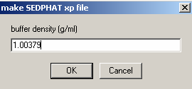
* from buffer composition (using SEDNTERP): buffer density =1.00379 and buffer viscosity = 0.010267
* from the amino acid composition of the protein (using SEDNTERP), the theoretical Mw of the protein is 8869 Da, the molar extinction coefficient (at 280 nm) = 8480 and the partial specific volume (V-bar) is 0,743
* using the DNA sequence and one of the many Oligo analysis tools on the web, we found the theoretical molecular weight of the DNA = 14087 Da and the extinction coefficient (at 260 nm ) of the DNA = 449100.
We did not observe any problem with the wavelength inaccuracy of the XLA, mostly probably because of the shallow gradients of the absorbance profiles where we measured (always stay with maxima or minima), and for 230 nm because the monochromator window is wide enough for the strong emission line of the lamp to pass through even if it is one or two nm off. (This may depend on proper wavelength calibration. If you experience a problem, maybe try to do an intensity wavelength scan from 200 to 250 nm on an empty cell, and determine the intensity maximum, and chose that as your far UV wavelength.)
Summary of Step 1: Loading and sorting data in SEDFIT
(Note there is a tu
In this section, it is shown how all the sedimentation equilibrium (SE) scan data from our run is opened in SEDFIT , sorted and saved as xp file ready for SEDPHAT. SEDFIT will save one .xp file for each wavelength per cell, for example, Cell1_280.xp Even if there has been several scans made during the approach to equilibrium, SEDFIT will select the latest scan, which will be used here to ensure that the data is in equilibrium (or as close as possible). When opened, each .xp file contains several scan patterns, one for each speed. In addition to .xp files, .RA (absorbance) files renamed to contain rotor speed and wavelength information in the filename will be saved.
SEDPHAT organizes the data in 'Experiments', which are objects that consist of the information of the experiment type, location of the data and list of data filenames, buffer conditions, sample extinction coefficients, some centrifugal parameters like meniscus, bottom, fitting limits, expected standard deviation, etc.
http://www.analyticalultracentrifugation.com/sedphat/experiment1.htm
This step in more detail
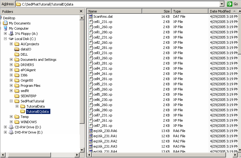
Open SEDFIT (not SEDPHAT yet). From the Sedfit window, go to “load new files” under the Data top menu.
Select the correct file location.

Open all the Ra scans from the SedEquil experiment at once by highlighting the first scan, holding down the “shift” key, highlighting the last Scan and clicking the Open button. Here, we open 630 scans total (90 scans each from the 7 cells of the Sed Equil run).
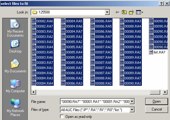
Load every file (answer '1' to the prompt 'load every n'th file').
[If you have collected intensity scans during the experiment, then select all "ri" scans (there will be no "ra" scans). You can also do the same thing with all "ip" scans if you have worked with interference optics.]
For more detail about loading data from Sedfit, go to:
http://www.analyticalultracentrifugation.com/sedfit_help_LoadNewData.htm
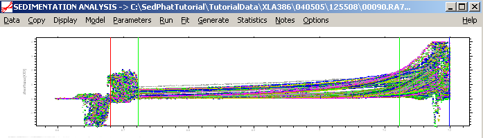
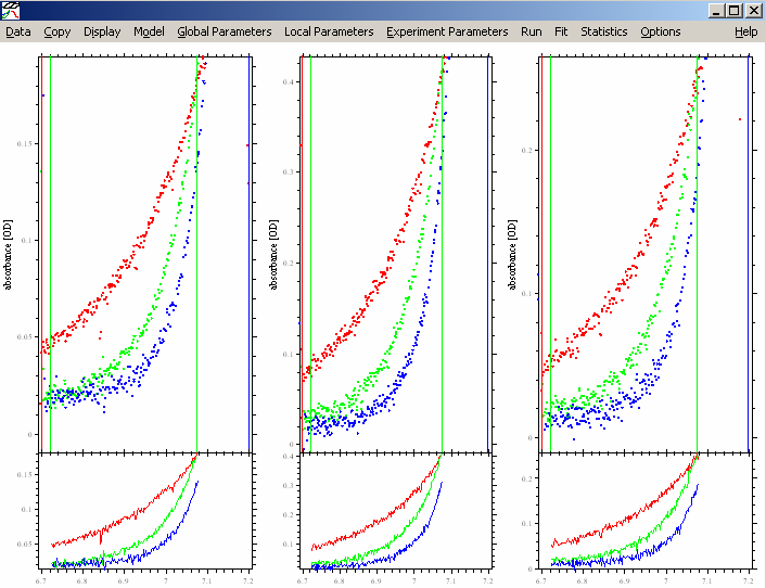
The pattern below shows all Absorbance scans opened at once with the meniscus (red) and the bottom (blue) limits of the solution column set. This will be fine-adjusted later. Then, set the inner (left green line) and outer limits (right green line) to mark the data analysis limits. At this point, this will get the limits simply in the ballpark, they will be adjusted later for each experiment. [As an alternative, if we had loaded only data from one cell, we could do the fine-adjustment here. This can be a good idea, for example, when dealing with the intensity data.]
For more details about setting limits, go to:
http://www.analyticalultracentrifugation.com/sedfit_help_LoadNewData.htm
Then, from the Sedfit “options” top menu go to “loading options” and click on “Sort Eq Data". (More general information on this function can be found here)
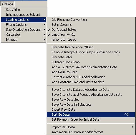
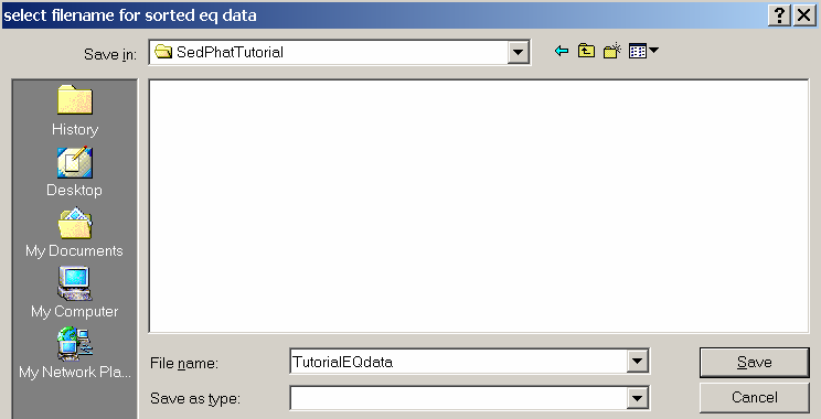
A files window will open, so select a location and filename and hit “Save” to save and sort the Eq data.
For the purpose of this tutorial, we create a directory c:\SedphatTutorial\TutorialEQData
A message appears asking you to make xp files - always answer yes to this question since we're going to analyze the data in SEDPHAT and use these xp files.

Then, a series of windows will appear. First, buffer density.
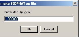
If you know your buffer density from SednTerp, enter it here:
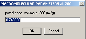
Next, partial-specific volume.
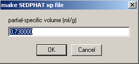
Enter 0.743 - the value from SednTerp calculated from the amino acid sequence for the protein. This does not seem right, because we're dealing here with the DNA. However, what counts is the buoyant molar mass, and entering different values for v-bar will simply shift the scale of the apparent molar mass. Since the buoyant molar mass is additive during for complex formation, the apparent molar masses of the protein and DNA will also be additive, if we calculate everything on the same v-bar scale. Otherwise, all species, including the complexes, will have different v-bars, which is difficult to keep track of. The downside of calculating with everything on the same vbar scale is that if we wanted to know the true molar mass, the apparent molar mass has to be converted using the partial-specific volume of the species in question. The advantage is that this way, we don't have to worry about the v-bar values.
Note also that here we don't really know the vbar of the DNA. It could probably be predicted using the base composition, but this procedure introduces errors similar to the prediction of vbar of the protein. What we're going to do here is to simply pretend we know the vbar, and then determine the apparent molar mass of the DNA and the protein. We'll double-check later that these are reasonable values.
This issue is explained in more depth in http://www.analyticalultracentrifugation.com/sedphat/partspecvols.htm.
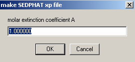
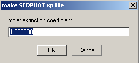
The next two windows ask for molar extinction coefficient of A and B. Use the default values here. Later while
entering experimental parameters, these values will be entered according to wave length
Hit OK
Hit OK
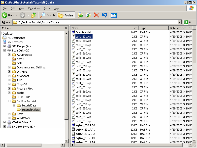
With all this information, Sedfit will proceed and generate a series of new files comprising the 'sorted' Eq data. This means Sedfit will save into the new folder only the latest scans at each wave length for each cell i.e. the ones that are in equilibrium. Notice that the RA files also include the speed and the acquisition wavelength in the filename. This facilitates the identification of files.
The xp files will bundle the scans taken from the same cell at the same wavelength into a multi-speed sedimentation equilibrium structure, which can be loaded directly with SEDPHAT.
This is how this should look like (using the Windows Explorer [which you may want to set up to see the file details]):
This concludes Step 1, and the preparation of the SE scans for analysis.
II) analysis of the DNA with a non-interacting single-species model
Summary of Step 2: Selecting the .xp files from Cell 1, and opening in SEDPHAT
We are going to load the first three xp files; all from cell 1 (contains 1 component, DNA), each taken at a different wavelength. Load each xp file by highlighting and hitting the open button. They will appear in the Sedphat window one at a time, from left to right, as they are loaded. In this step, we will also set the fitting limits and meniscus and bottom.
In more detail:
First, open SEDPHAT
From the Sedphat window, under the top menu” data”, go to Load experiment.

Find the folder containing your Sorted EQ data.

Highlight the first file (here cell1_231.xp). After loading the first .xp file, a window will appear with the v-bar value that you entered previously.
Hit Ok.
You will need to re-enter this data later when adding experimental parameter values.
After that, load the second file (cell1_260.xp) and the third (cell1_280.xp).
An alternative way to load xp files is to open Windows Explorer and just drag and drop the file cell1_231.xp into the Sedphat window.
![]()
After the first file is open in SedphaT, the window asking for the global v-bar value appears.
Like above, enter the value for the protein. Hit OK. (More later on the fact that we’re looking at the DNA, and the vbar is that of the protein.) Now, load, by dragging and dropping, the second data set. This will be cell1_260.xp. Then load the third, which is cell1_280.xp.
Either way, we end up the the following picture, showing all the xp files for cell 1, at the different wavelengths. We have loaded all 3 wavelengths from cell #1 of the Sed EQ run. Also notice that each experiment (each wavelength), contains 3 scans, one at each speed. In this case, 16k, 24k and 30k.
Next, adjust the meniscus and bottom of the solution column if needed and adjust the inner and outer data limits, making sure the outer data limit stays < 1.5 OD. This works exactly the way as in SEDFIT, except that you click with the mouse into the section on the screen of the respective experiment. If you’re not familiar with that, please go back to the SEDFIT tutorials. Specifically, for more details about setting limits, go to: http://www.analyticalultracentrifugation.com/sedfit_help_LoadNewData.htm
Then, from Display,” show last fit info again” or hit control –O to show identity of each file.
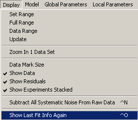
This will also show the setting of the default SEDPHAT parameters in the default model (not fitted yet.)
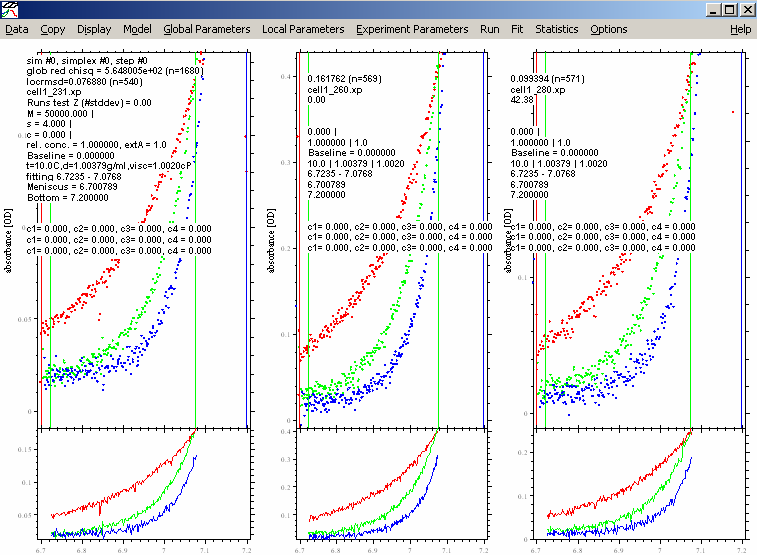
In order to update the experiments with the settings for the fitted limits, use the function
Data->Save All Experiments.
This will copy the current fitting limits into the xp files on the hard drive, so that they will be restored the next time you load the experiments. Generally, be aware that files on the hard drive and memory state of SEDPHAT are different things, and changes in the SEDPHAT window are not updated to the files unless you explicitly request this.
Summary of Step 3: Choosing a model and setting up parameters for a first fit
After all files are loaded and you are happy with the placements of the data limits, it is time to set up the configurations for the analysis. We begin by choosing a model and then, follow along the top menu to adjust global parameters, local parameters and experimental parameters. These describe properties of a particular experiment, like loading concentration, baseline parameter, meniscus position, but also the extinction coefficient at the particular wavelength used. In SedPHaT, the local parameters are subdivided in the concentration parameters, accessed in the Local Parameters menu, and the Experiment Parameters, which contain those related to the physical setup of the experiment.
For more Parameter information, go to: http://www.analyticalultracentrifugation.com/sedphat/parameters1.htm
In this case, we choose the monomer-dimer self-association model.
This Step will also describe how to set up the links between experiments: Since we're looking at xp files from the same cells at different wavelengths, we will link all bottom parameters to one, link all concentration parameters to one, and we can float all but one extinction coefficients.
In detail:
Go to the function Model->Monomer-Dimer Self-Association

(Don’t panic - we’ll fit only a single species, but are going to use an interacting model in order to exploit the mass conservation features and express the fit in molar concentrations.)
Then, open the parameter box by using the menu function “Global Parameters”:
![]()
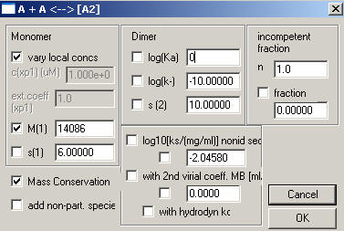
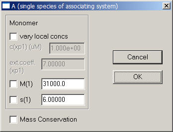
Here, we enter the theoretical MW of the monomer, in this case DNA, turn on the mass conservation (check the box to the left of ‘Mass Conservation’) . Default the rest. Turn off the Dimer (un-check) and enter 0 for log(Ka), this will change this model to represent the monomer only. The S values are insignificant, we are looking at equilibrium data. (just make sure they are not floated, i.e. make sure they are un-checked). Hit OK.
[In future versions (4.0 and later), there will be an extra model for a monomeric species, which does not require using the monomer-dimer model at log(Ka)=0. Otherwise, it will have the same functionality for the present purpose.]
Next, use the function Local Parameters from the top menu.
![]()
In the local parameters, the concentration of the single species is entered for each experiment through a series of windows. Since we are looking at the same AUC cell (cell 1) here, we can link the concentrations of experiments # 2 and # 3 to exp #1 in the following windows when asked. This tells the program to take only a single value for the concentration of cell 1.
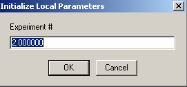
This is how this is done: Start with Experiment # 1.
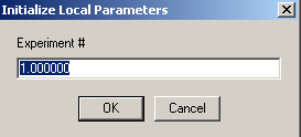
Experiment 1 will serve to hold our concentration parameters, so we will not redirect it: 'concs of exp #1 linked to exp # 1'
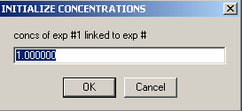
Next, enter the loading concentration of DNA (an estimate will do at this stage).

Link the concentration of exp # 2 to experiment #1 from the following 2 windows:
For Experiment # 2:
Specify that the 'concs of exp#2 will be linked to exp# 1'
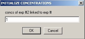
As mentioned above, this will direct SEDPHAT that exp# 2 will not have an independent concentration parameter, since it is the same cell as exp# 1.
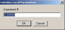
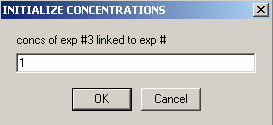
Similarly, link the concentration of exp # 3 to experiment #1:
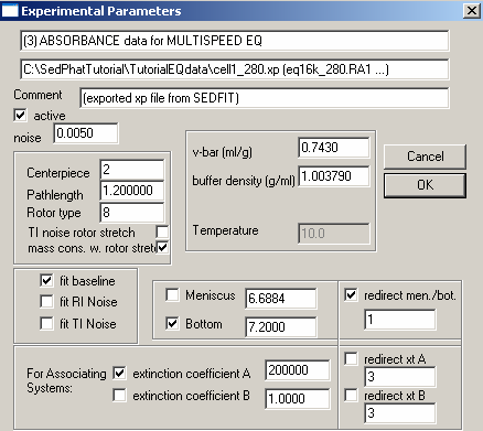
Now, the individual experimental parameters for each
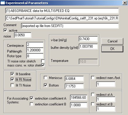
experiment will be set up. Go to Experimental Parameters on the top menu.
![]()
This window will appear:
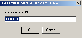
Let's start with the first experiment. Hitting OK here will display the parameter window (below) for exp # 1.
 l
l
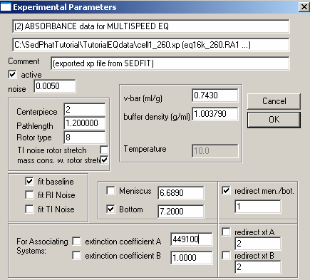
Look at the lower section for the extinction coefficients: Experiment # 1 is at wavelength 230 - enter a starting guess. Just from looking at the raw scans, it appears that the 230 absorption is little more than 1/2 of that at 260 nm, so we enter half the value of the extinction coefficient at 260 nm. But we don't know it exactly, therefore we will check this parameter, so that it will be floated and optimized in the fit.
Next, look at the middle section on the left dealing with the rotor: we will fit for “mass cons.w.rotor stretch". This will take into account that at different rotor speeds the rotor stretches, which changes slightly the mass balance across the cell.
In the middle, check the field for the bottom. Fitting for the bottom position is very important, since mass conservation analysis integrates from meniscus and bottom, but we don't know exactly where the bottom of the cell is. [If you don't use mass conservation analysis (see the global parameter window shown above), then you don't need to float for the bottom of the cell.] These issues are described in Analytical Biochemistry 326:234-256 (preprint). We don't fit for the meniscus position, because it is far less important for mass conservation analysis.
Double-check the following parameters:
* V-bar value 0.743 Note that the v-bar value is that of the protein (see above)
* Buffer density 1.003790
* Centerpiece: 2 – (double-sector centerpiece)
* Pathlength: 1.2 (standard 12mm thickness centerpiece)
* Rotor type: 8 (8-hole rotor An 50 TI)
* Fit baseline is checked as default, but the other fits i.e. RI noise, TI noise, are options.
After parameters are in place, hit the OK button and these windows will appear:
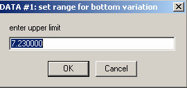
OK them both. This is the default variation allowed for the bottom position.

That will bring us to exp #2.
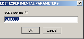
As before, the experimental parameters window for experiment # 2 will appear.
For exp #2 at 260 nm, the theoretical extinction coefficient is entered, as found from the DNA sequence. It is fixed (not checked). This is because we know this value from the sequence, and will use it to scale the concentration values. [Later, the concentration value will be floated in the global fit. We cannot float simultaneously the concentrations and all extinction coefficients. Since we’ll linked the concentration values of all xp files, we can float all but one extinction coefficient. Since we have to keep one extinction coefficient fixed, and the obvious choice is to do this in the experiment at 260 nm, since here we have a theoretical extinction coefficient value.]
For the bottom: Put a checkmark next to the bottom field to fit for this parameter. Note, however, in this case, we redirect the bottom to exp #1 (since it is the same cell) by checking the box "redirect mem./bot."and entering 1 in the box underneath it. This uses the constraint that one cell has only one bottom position, and we don't need more then one parameter to describe it.
Here also, we fit for mass cons.w.rotor speed. And again, also double-check the following parameters:
* V-bar value 0.743 Note that the v-bar value is that of the protein (see above)
* Buffer density 1.003790
* Centerpiece: 2 – (double-sector centerpiece)
* Pathlength: 1.2 (standard 12mm thickness centerpiece)
* Rotor type: 8 (8-hole rotor An 50 TI)
* Fit baseline is checked as default, but the other fits i.e. RI noise, TI noise, are options.
Hit OK and this window appears:

Hit OK, to get to exp #3

and the parameters window.
For exp #3, the extic coeff is entered at about ½ that of wavelength 260 (exp#2), a starting estimate obtained just from looking at the scans (we get about half the OD values at corresponding radii and rotor speeds). We fit for mass conservation and again, the bottom fitting is directed to exp #1. Specify everything else as shown and described above.
Hit OK
Summary of Step 4: Save configuration
The combination of a set of experiments, the model, the model parameters, and the links between the experiments and shared parameters is termed 'configuration'. By saving configuration files, we have a starting point to later change models or re-enter new parameters.
For more info about configurations, go to:http://www.analyticalultracentrifugation.com/sedphat/configurations.htm
To do this, from the top "Data" menu, go to "save current configuration as".
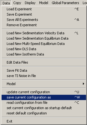
Select a folder and name for this initial configuration.
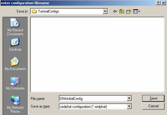
Always answer "Yes" to this question

(it will leave the old xp files intact - just in case we need to come back to them at a later point, perhaps they are being used by a different configuration).
As shown in the Windows Explorer, this function creates a bunch of files:
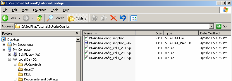
These are a file "*.sedphat" that describes the complete state of the analysis. The information in the sedphat-file are the paths of all the experiment files (xp-files) loaded, the global parameters like vbar(20), and all links between local parameters of the experiments. It will also automatically write a "*.sedphat_PAR" file with the type and global parameters of the current model.
Because sometimes you may want to make different analyses of the same data with different models, and because different models may change the local parameters stored in the xp-file (like meniscus position, etc.) it is advisable to make a new copy of the current xp-files for each configuration. That way, the complete information about the analysis can be stored in a reproducible way, and several alternative analyses of the same data may co-exist.
You can load a previously saved configuration into Sedphat by dragging-and-dropping a 'sedphat' file into the Sedphat window from Explorer. Sedphat will automatically load the 'sedphat'-file and its associated 'sedphat_PAR' data.
After saving, have a look at the title bar of the Sedphat window:
![]()
It will now reflect the name of the current configuration. Note that much of the information stored relies on the exact location of your xp-files and the sedphat_PAR file on your computer. If you move your analysis between different computers, it is best to use exactly the same directory structure. Alternatively, you can edit the sedphat files with the notepad and adjust the pathname of the xp and the sedphat_PAR files.
Do not use directories with white-space characters, e.g. "My Documents", "XLA DATA" or the desktop. The keyboard shortcut is control-W.
You can load a previously saved configuration into Sedphat by dragging-and-dropping a 'sedphat' file into the Sedphat window from Explorer. Sedphat will automatically load the 'sedphat'-file and its associated 'sedphat_PAR' data. OR....go to Data >>read configuration from file. This is a way to restore a previous SedphaT configuration and exactly reproduce an analysis. It reloads the data, the model, the global parameters, and restores all links between the data sets. Be aware that the file structure is important (see above), otherwise SedphaT won't find the data. The keyboard shortcut is control-C
[Note addition from version 4.0 and later: There is a new function "copy all data and save as new config", which will create copies of all the raw data files, xp files and configuration files, and store them in a new folder without absolute path names. This makes it easier to document, move, and archive an analysis.]
Summary of Step 5: Run and Fit
Background: SedPHaT makes the same distinction between "Run" and "Fit" as in SedfiT. In brief, the Run command executes a model, i.e. it performs a simulation using the parameters values that were entered as starting guesses in the global, local, and experimental parameters section. It does optimize all linear parameters, which do not require starting guesses, but does not optimize the (usually more difficult) non-linear parameters.
The importance of the distinction between "Run" and "Fit" is that for non-linear regression, one needs good starting estimates for the nonlinear parameters. Without them, the fit can frequently converge in local minima, and the best-fit may not be found. There is no good alternative to just ('manually') exploring different parameter ranges, and position them so that they'll be able to converge to the overall best fit.
In the process of exploring the parameter space, you will need to assess what the current parameter values do to the model. This is done with the Run command. See also The difference between 'run' and 'fit' in sedfit
and http://www.analyticalultracentrifugation.com/sedphat/run.htm
In SedPHaT, you can start the non-linear regression for a single experiment or for all of them. Limiting the regression can sometimes be useful at a first stage in order to converge parameters for which a particular data set has very significant information without swamping it with the data from all other experiments. It can also be useful to converge the local parameters (such as local concentrations), before doing a global fit, to avoid poor initial estimates of local parameters throw off the global parameters.
You can interrupt a fit by pressing any key. This will execute the model for the so far best parameters found. (Don't press a key twice in a short interval, in order not to abort the calculation of the so far best model.)
This is how this is applied here:
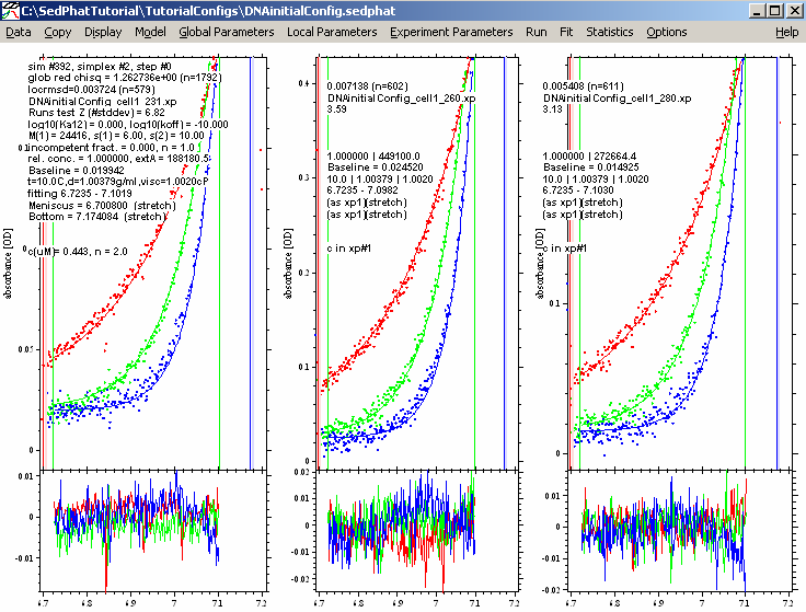
From the top menu, execute a global run from:
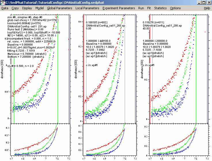
Below are the results of the Global run.
(If the window does not look like that, try to use the function Display->Data Range, which zooms in to show the fitted data best.)
This is obviously not a great fit, but it is good enough for what we are looking for at this stage: The fitted curves (lines) have shapes similar as the data. Even though they don't match well, yet, this is a good starting point.
Now we will do a fit:
[It can be advantageous to begin with a Nelder-Mead simplex optimization, by making sure that 'Marquardt-Levenberg' in the Fitting Options is unchecked.

For more fitting information, go to: http://www.analyticalultracentrifugation.com/sedphat/fit.htm]
Select the function Global Fit from:

This will start the fit, during which you will notice the parameter numbers change. In particular, you can look at the 'locrmsd' fields and see the error of fit decrease.
[During the fit, if you have specified a configuration filename, a new set of "*.sedphat" files and "*.sedphat_PAR" files (and copies of the xp-files) was generated that stores the so far best intermediate results during the optimization. These files will be preceded by '~'. This enables the restoration of the so far best fit in case the optimization crashes later on or is lost for some reason.]
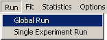
1st Fit results:
Not a bad fit at all. The global reduced chi-square number is 1.26. In the usual meaning, it would be 1.00 for a perfect fit, but this depends on the correct estimation of the experimental noise (the field in the upper left corner of the Experiment input boxes), which we usually don't know very well. Therefore, we use this only as s relative measure.
But try to make it better by fitting for RI noise. This is time dependent/radial independent noise that takes into consideration that the baseline changes with rotor speed but generally remains flat. The reason for choosing this option here is the fact that the residuals of the first experiments are all flat, but offset vertically relative to each other, indicating a possible baseline issue.
To do this, from the experimental parameter top menu, edit all 3 experiments and fit for RI noise in each experimental parameters box:
Starting another global fit produces these results:

A better fit here...notice the reduced chi squared is now 1.139, and the rms error values are a bit better.
Now, to be sure that we have found the global best-fit, we switch to the Marquardt-Levenberg method:

(leave the “Fit M and S” alone - this should remain checked). The Marquardt-Levenberg method has a way to better home in to the best-fit when close to the optimum.
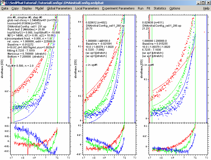
This results in:
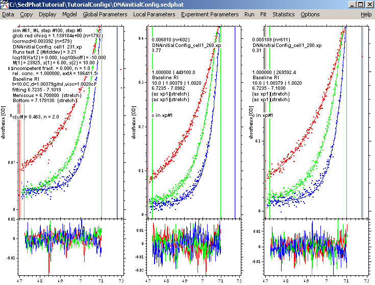
This is virtually the same as before in the Simplex fit, showing that we are in the overall global best-fit.
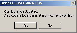
We will save this result to the hard-drive, so that we can always restore this fit. Choose 'update current configuration':
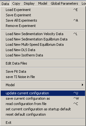
Yes! Update the xp files also.
Step 6: Interpreting the Result
There are a couple of things we are looking for.
1) We notice the fit quality is excellent. The residuals are pretty random and small. This will give us confidence in the numbers. To be sure, we should also conduct a rigorous analysis of the error limits for each parameter - and we'll show how to do that in the analysis of the mixture - but the model of a single monomeric species is simple enough that we won't need to worry about it at this point.
Another interesting point to note here is that there is no reason to believe mass conservation is not valid. This supports using mass conservation also when analyzing the mixture.
2) Look at the Mw value of 23.9 kDa. This is quite a bit higher than the initial estimate, which we took as the true Mw from base sequence. However, this is only an apparent molar mass, on the v-bar scale of 0.743. The buoyant molar mass is 23.9*(1-0.743*1.0038) = 6.07 kDa. This is the only relevant quantity for sedimentation. Knowing that the true molar mass of the oligo is 14.1 kDa, we can calculate the vbar as vbar = (1/1.0038)*(1-6.07/14.1) = 0.57 ml/g, which is in the range of vbar values known for nucleic acids. (The lower value 0.57 ml/g means nucleic acids are much more dense, i.e. they displace less water and have lower buoyancy, and therefore their apparent mass on a v-bar scale of the protein appears much higher than their true mass.)
For the interaction to be studied, the apparent mass of 23.9 kDa will be the value we use, in conjunction with the v-bar value of the protein of 0.743.
3) The extinction coefficients are 449100 OD/Mcm at 260 nm (this was fixed to the theoretical value), 186,400 OD/Mcm at 230 nm, and 269,600 OD/Mcm at 280 nm. These values will also be used as fixed prior knowledge for the multi-wavelength analysis of the mixture of DNA with protein.
go to next step - analysis of the protein with a non-interacting single-species model