
back to the start of the tutorial
III) Analysis of the protein with a non-interacting single-species model
The third step of this tutorial is the characterization of the protein by itself. The data are as described before. The protein by itself is in cell 2 of the run. We also have already used Sedfit to prepare the SE raw data files and generate the xp-files for all cells. We don't need to redo this. Therefore, we jump directly to the next step, loading the protein data into a new Sedphat window.
Step 7: Selecting the .xp files from Cell 2, and opening in SEDPHAT
We are going to load the first three xp files; all from cell 2, each is a different wave length. From the Sedphat window, go to "Load Experiment" from the Data top menu. Locate your .xp files and load each xp file by highlighting and hitting the open button. They will appear in the Sedphat window one at a time, from left to right, as they are loaded. When linking data, this order of loading is something to take into consideration.
In detail:
Open a new Sedphat window and select:

Here, we begin the loading with cell2_281.xp (the scans are taken at 280 wavelength),
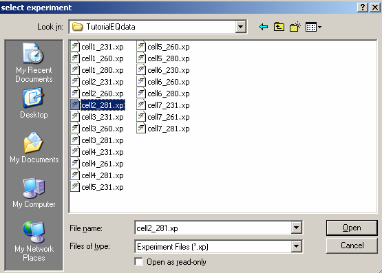
Select 'Open'. After the first file is open in SedphaT, the window below appears.
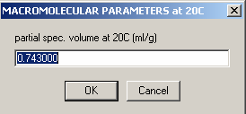
Here, the v-bar value (from the amino acid sequence) that you entered earlier while “sortingEQ data in Sedfit is displayed. Hit OK.
Then load cell2_260.xp, then finally cell2_231.xp. Highlight each .xp file one-at-a-time and "Open". They will appear in the Sedphat window in the order that they were loaded from left to right.
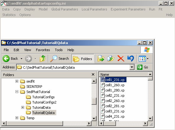
As an alternative loading style, you can drag and drop files from Explorer. Below, Explorer is opened and the .xp files are dragged from Explorer into the Sedphat window space one at a time.
After all three .xp files from cell #2 have been loaded (below), notice that each experiment (each wavelength), contains 3 scans, one at each speed. In this case, 16k, 24k and 30k. Each experiment has a number associated, which is the order of loading. This will be the same as the order of the plots from left to right in the Sedphat window (upper row before lower row). Many Sedphat functions operate on specific experiments, and the user has to specify the corresponding experiment number.
In order to see the data at a better magnification, use Display->Data Range (or keyboard shortcut Control-D). This will make it appear larger:
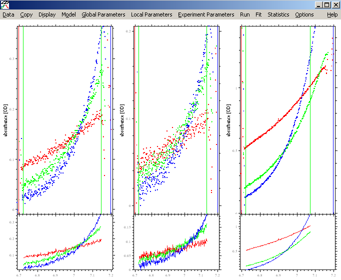
Adjust the meniscus and bottom of the solution column if needed and adjust the inner and outer data limits, making sure the outer data limit stays < 1.5 OD. This works exactly the same way as in SEDFIT, except that you click into the section on the screen of the respective experiment. If you're not familiar with that, please go back to the SEDFIT tutorials. For more details about setting limits, go to: http://www.analyticalultracentrifugation.com/sedfit_help_LoadNewData.htm
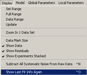
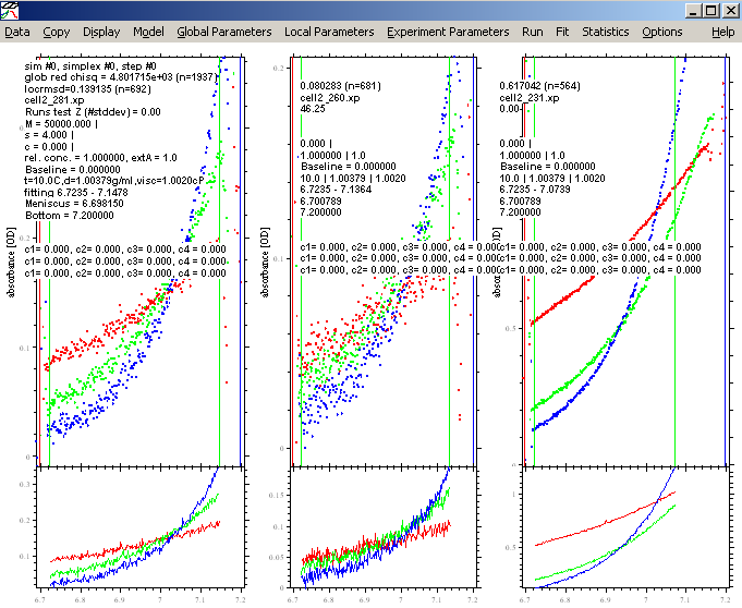
Then, from Display, "show last fit info again", or hit control-O to show the identity of each file.
This will also show the setting of the default Sedphat parameters (not fitted yet) as in the window below.
In order to update the experiments with the settings for the fitted limits, use the function Data>Save>All Experiments.
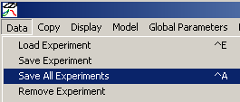
This will copy the current fitting limits into the xp files on the hard drive, so that they will be restored the next time you load the experiments. Generally, be aware that files on the hard drive and state of SEDPHAT are different things, and changes in the SEDPHAT window are not updated to the files unless you explicitly request this.
Step 8: Choosing a model and setting up parameters for a first fit
Summary: After all files are loaded and you are happy with the placements of the data limits, it is time to set up the configurations for the run. We begin by choosing a model, then follow along the top menu to adjust global parameters, local parameters and experiment parameters. These describe properties of a particular experiment, like loading concentration, baseline parameter, meniscus position but also the extinction coefficient at the particular wavelength used. Like before for the DNA, in this case, we choose the monomer-dimer self-association model. At this stage we will also set up the links between the xp files loaded.
This Step will also describe how to set up the links between experiments: Since we're looking at xp files from the same cells at different wavelengths, we will link all bottom parameters to one, link all concentration parameters to one, and we can float all but one extinction coefficients.
In detail: Go to the function Model->Monomer-Dimer Self-Association

(Again, we’ll fit only a single species, but are going to use an interacting model in order to exploit the mass conservation features and express the fit in molar concentrations.)
Then, open the global parameter box by using the menu function “Global Parameters”
![]()
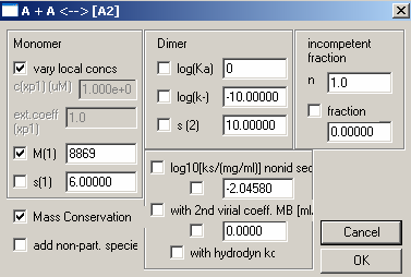
Here, we enter the theoretical MW of the protein monomer, fit for mass conservation (check the box to the left of ‘Mass Conservation’) . Turn off the Dimer (un-check) and enter 0 for log(Ka). Make sure nothing else is checked. The s-values are not significant because we are looking at equilibrium data. Then, hit OK.
[In future versions (4.0 and later), there will be an extra model for a monomeric species, which does not require using the monomer-dimer model at log(Ka)=0. Otherwise, it will have the same functionality for the present purpose.]
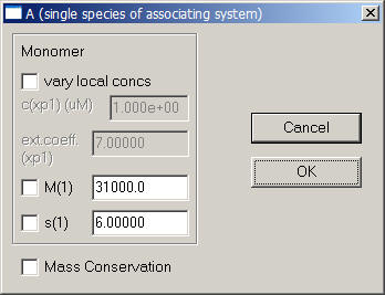
Next, use the function Local Parameters from the top menu.
![]()
In the local parameters, the concentration of the single species is entered for each experiment through a series of windows. Since we are looking at only Cell #2, we can link the concentrations of experiments # 2 and # 3 to exp # 1 in the following windows when asked. This will tell the program to take only a single value for the concentration of cell 1.
First, choose Experiment 1:
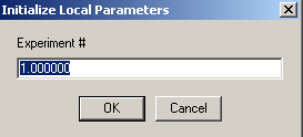
This will not be redirected, but contain our single concentration parameter, and therefore we link 'concs of exp #1' to exp # 1.
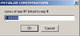
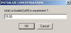
The concentration value we enter is our loading concentration of 15 microM.
Next, we go to experiment 2:
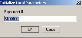
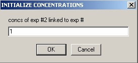
We link the concentration of exp # 2 to experiment #1, indicating that it is the same concentration (and allowing us to float the extinction coefficient instead).
Finally, go to exp 3
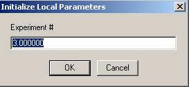
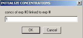
and link the concentration of exp # 3 to experiment #1
Now, the individual parameters for each experiment will be set up. Go to Experiment Parameters on the top menu.
![]()
This window will appear
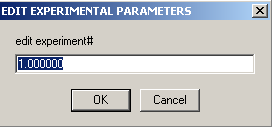
Hitting OK here will display the parameter window (below) for exp # 1.
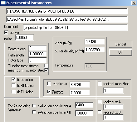
Experiment # 1 is at wavelength 280 so we will enter the theoretical extinction coefficient of the protein (from SedNTerp) and leave it fixed (un-checked). This will be our reference for determining the concentrations, and allowing us, in turn, to float the extinction coefficients at the other wavelengths.
We will fit for the bottom and mass conservation with rotor stretch. Check the following parameters: v-bar, buffer density, centerpiece (2=double-sector centerpiece), Rotor type: (8=8-hole rotor An50 Ti), Fit baseline is checked as a default, but the other fits i.e., RI noise, TI noise, are options.
After the parameters are in place, hit the OK button and these windows will appear:
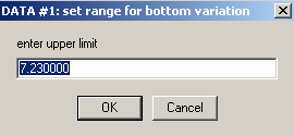
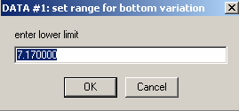
We will agree to these default limits on the variation of the bottom position.
This will open the window for the next experimental parameter box:
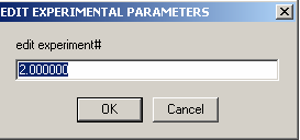
Then hit OK to open the Parameter box for experiment # 2.
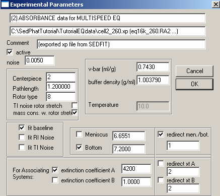
Experiment # 2 is at wavelength 260 so we will enter an extinction coefficient of about 1/2 of the one entered at 280 and we will fit for it (check the box to the right of it). Since we are looking at the same cell (just as we linked the concentration values) we are going to link the bottom and meniscus fitting to exp# 1. To do this, check the box to the left of either Meniscus or Bottom, the check "redirect men./bot. box on the right and underneath in the space, type 1. This will direct the meniscus and bottom of experiment # 2 to experiment # 1. Look at the other parameters as described above to make sure they match exp. # 1.
Then hit OK and this box will appear to remind you that the meniscus and bottom are linked to exp # 1. Hit OK.

Next, exp #3 windows appear. First:

Then, the parameters box for exp. #3:

Experiment # 3 is at wavelength 230 so we will enter an extinction coefficient of about 5 times that of 8480 (at wavelength 280) and fit for it (check the box to the left of it). Since we are still looking at the same cell, the bottom and meniscus will also be linked to experiment # 1 in the same way we did in exp. # 2. To do this, check the box to the left of Bottom, the check "redirect men./bot. box on the right. Underneath in the space, type 1. This will direct the meniscus and bottom of experiment # 3 to experiment # 1. Look at the other parameters as described above to make sure they match exp. # 1. Then hit OK. This reminder will again appear:

Hit OK.
Since setting up the fit and the links was a lot of work which we don't want to redo, we'll save the configuration.
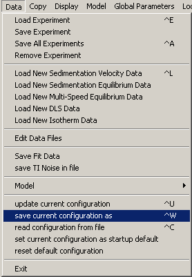
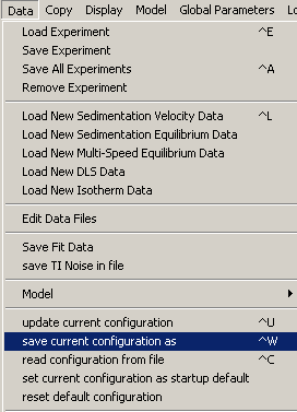
To begin, from the top "Data" menu, go to "save current configuration as".
Locate a destination folder and name this initial configuration.
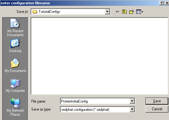
Generally, it is a good idea to answer "Yes" to this question

(this will make sure we won't override local parameters saved in the xp file.)
Now, the name of the current configuration file is shown in the title bar of the Sedphat window.
![]()
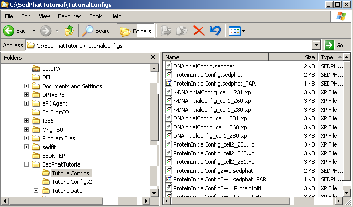
If we look at the contents of our 'TutorialConfigs' folder, we can see now set of new files containing the configuration that we've just saved.
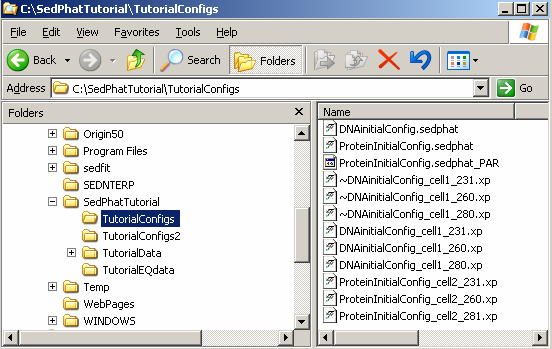
Note that much of the information stored relies on the exact location of your xp-files and the sedphat_PAR file on your computer. If you move your analysis between different computers, it is best to use exactly the same directory structure. Alternatively, you can edit the sedphat files with the notepad and adjust the pathname of the xp and the sedphat_PAR files.
[Note addition from version 4.0 and later: There is a new function "copy all data and save as new config", which will create copies of all the raw data files, xp files and configuration files, and store them in a new folder without absolute path names. This makes it easier to document, move, and archive an analysis.]
Do not use directories with white-space characters, e.g. "My Documents", "XLA DATA" or the desktop. The keyboard shortcut is control-W.
You can load a previously saved configuration into Sedphat by dragging-and-dropping a 'sedphat' file into the Sedphat window from Explorer. Sedphat will automatically load the 'sedphat'-file and its associated 'sedphat_PAR' data. OR....go to Data >>read configuration from file. This is a way to restore a previous SedphaT configuration and exactly reproduce an analysis. It reloads the data, the model, the global parameters, and restores all links between the data sets. Be aware that the file structure is important (see above), otherwise SedphaT won't find the data. The keyboard shortcut is control-C.
In order to get started, we double-check that our starting estimates get us reasonably close into the ballpark of the data.
From the top menu, execute a global run:

The result is this:
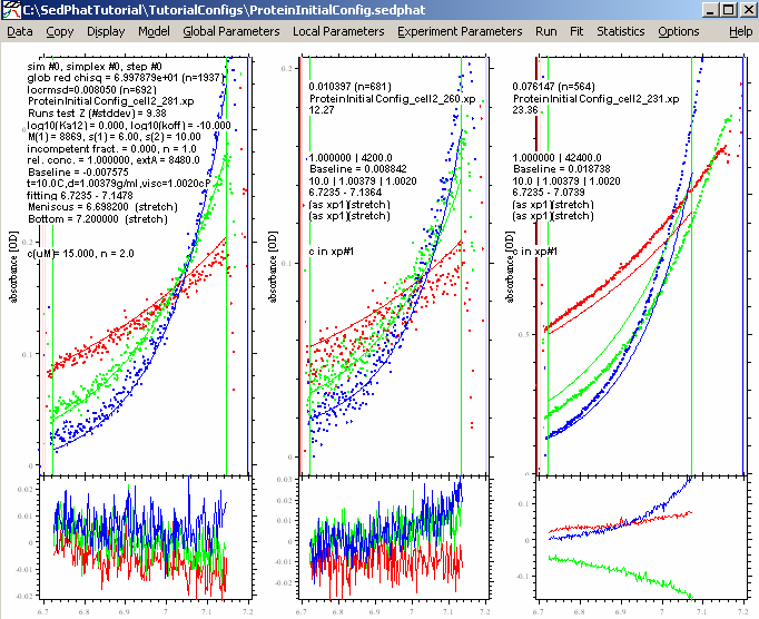
This seems to be pretty close to good values, certainly enough to start the non-linear optimization algorithms. First, we like to use the Nelder-Mead simplex optimization.

Then, start a Global Fit from:

resulting in:
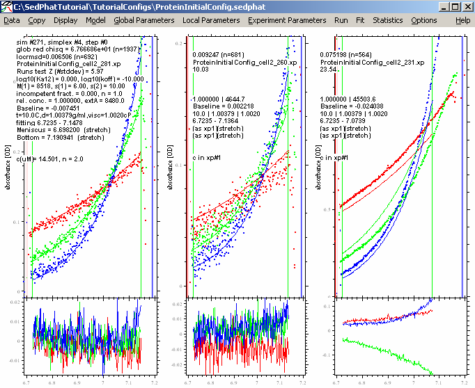
For the data at 280 and 260 nm, the fit looks pretty good, but not for the 230 data (at the right). We can try (like with the DNA) to make it better by fitting for RI noise (i.e. allowing for a rotor-speed dependence of the baseline), and by bring in the outer data limit for exp #3 in a bit (just in case the scan is too steep or the data are getting into a non-linear range - although this generally shouldn't be the case as long as we're at OD < 1.5). For RI noise fitting, go back to each experiment parameters box and check RI noise as in the window below:
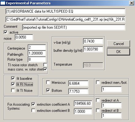
Do this for all cells. Performing another Global Fit gives us these results:
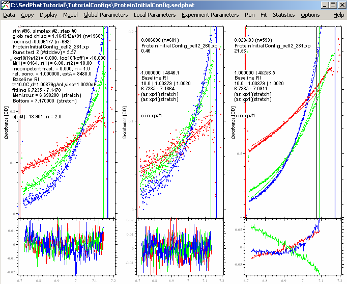
This is a better fit, but experiment # 3 still looks bad. It is possible that we have some low molecular weight impurity in the sample, perhaps a degradation product of the protein, which does not absorb at 260 or 280 nm but does contribute to the signal at 230 nm (maybe a peptide without aromatic amino acids). For the analysis, we won't need the 230 nm data, since two wavelenghts will be enough to discriminate the protein and the DNA.
Therefore, to see what the fit would be without it, we can go into exp # 3 experiment parameters and make it inactive. Before doing that however, update this configuration by going to the following menu
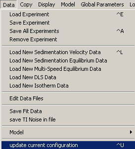
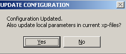
This window appears...ALWAYS say "Yes" to this question.
Then, to inactivate exp #3, from the top menu choose Experiment Parameters
![]()
, edit experiment # 3

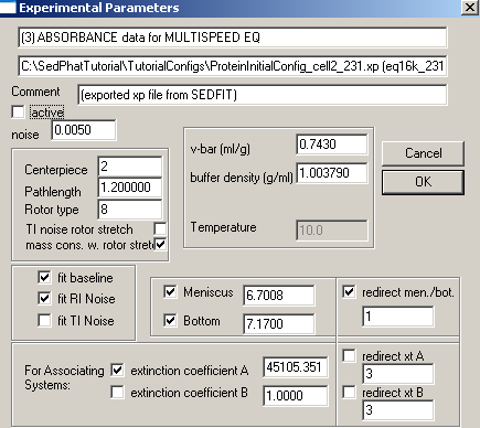
and get to the parameters window. Just under the comment line, there's a small check box beside "active". By un-checking this box, experiment # 3 will become inactive (i.e. temporarily not be considered in the fit, although drawn in the sedphat window).
Then do another global fit with experiment # 3 inactive:
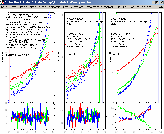
Now, the rmsd values for the 280 and 260 data are great, and the fits appear perfect. We decide to leave out the 230 nm data.
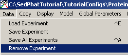
Remove exp #3 completely from the configuration this way: First from top menu go to Data>Remove Experiment
select experiment # 3
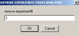
After hitting OK, this window appears; a reminder to re-link the concentrations and the meniscus/bottom fitting of exp #2 to exp #1.

The concentration and meniscus/bottom fitting links will have to be reestablished between exp #1 and exp #2. To do this, go back to Local parameters in the top menu to re-link the concentration in experiment #2 to exp #1 and then to the experiment parameter to re-link the meniscus/bottom fitting in exp #2 to exp #1. To see this in detail, please refer to Step #3 of this Tutorial. After removing exp #3, notice that the title bar of the new configuration is blank (since it was changed).
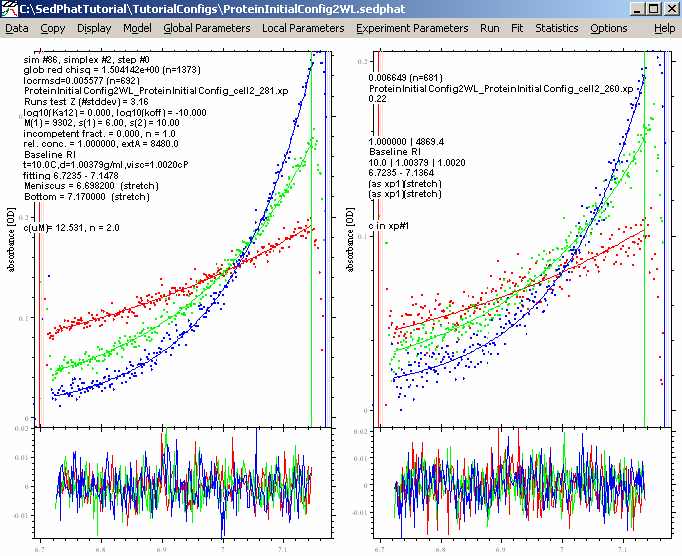
Now do a new fit:
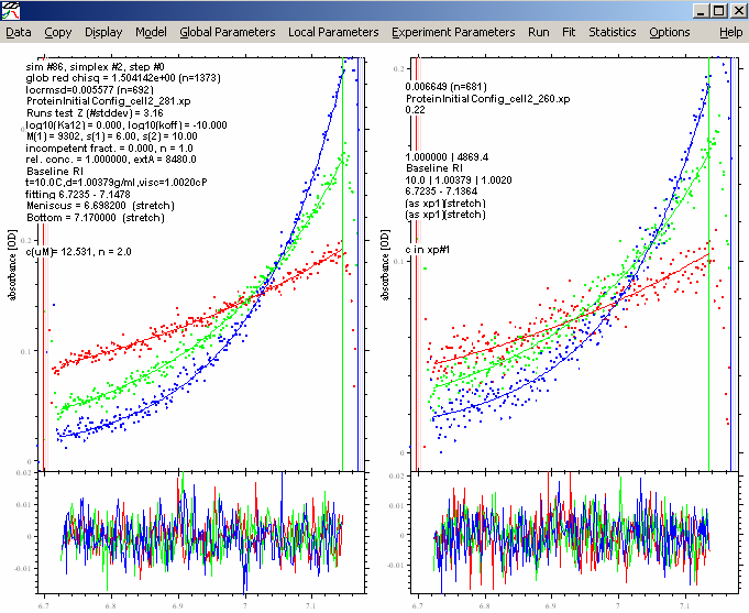
This is the same as we had with the 230 nm data inactive. Save this configuration with a new name.
To the question

answer yes.
A look into our TutorialConfigs folder shows us all of the configuration files so far.
After saving the last configuration, notice that the new file name is now in the title bar.
Although we had a very good fit, we should make sure that we're really in the global optimum. Therefore, we fit again using the Marquardt-Levenberg algorithm to home in on the optimum. Under the "Option" top menu go to "Fit Options" and toggle on the Marquardt-Levenberg fit. (Don't touch the "fit M and s" fitting option.) This will look like this:

Then repeat a Global Fit

Compare these results with the previous fit and they look very much the same. So, consider this the best fit and update the configuration:

and the .xp files

Step 11: Results for the Protein
Note the following points:
1) The fit quality is excellent. The residuals are pretty random and small. This will give us confidence in the numbers. As for the DNA before, there is no indication to believe mass conservation is not valid. This supports using mass conservation also when analyzing the mixture.
2) The Mw value is 9.3 kDa. This is slightly higher than the theoretical Mw of 8.7 kDa. The v-bar used was 0.743 ml/g, which is correct for the protein, and therefore the observed Mw should be identical to the theoretical Mw of the protein. Nevertheless, either the Mw value is 7% too high, or, correspondingly the true vbar value is 0.726 ml/g ( Mb = 9.3*(1-0.743*1.0038); vbar = (1/1.0038)*(1-Mb/Mtrue)). This deviation could be within the error of the prediction of vbar from amino acid sequence (because the larger surface/volume ratio, the error in the tabulated vbar is larger for smaller proteins). Alternatively, we could be dealing with a contamination with a few percent of protein aggregate. At this stage, it is usually a good idea to check the c(s) from a sedimentation velocity experiment to see if there was any evidence of such contamination. If not, this is within the usual range of precision, and we will accept the value of 9.3 kDa (and use it in the analysis of the mixture), continuing to use 0.743 ml/g as our vbar scale.
3) The extinction coefficient are 4868 OD/Mcm at 260 nm, and 8480 OD/Mcm at 280 nm (this was fixed to the theoretical value). These values will also be used as fixed prior knowledge for the multi-wavelength analysis of the mixture of DNA with protein.
go to next step - analysis of the mixtures