back to the tutorial main page
Loading the data and preparing the analysis
Load the complete data set into Sedfit. A detailed description on how to load data can be found here. Initially, the Sedfit window will look like this:

with the data plot on top, and the residuals plot below initially showing the same data.
NEW in version 11.0 and higher: The default color scheme is scaled such that the first scans are black/blue and the last scans are deep red.
All colors should be visible after loading the
scans. (When loading other data sets where some of the scans are very late
in the run such that virtually only superimposing baselines are scanned in the
final scans, the red colors will all superimpose and be hardly visible.)

Please note that the sedimentation was not recorded to completion; for this sample under the conditions of this run, approximately 200 scans instead of only 130 would be required for an optimal analysis. In general, it is highly recommended to include a data set as large as possible.
As a next step, select the bottom, meniscus, and the outer and inner fitting limits. How to do this is described in very detail in the help section for the menu on how to load new files.
For this particular sample, I would set the limits as shown here:

(After entering the fitting limits, the residuals plot switches to show all the data between the fitting limits.)
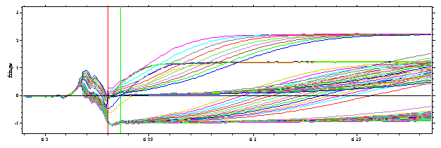
By spanning a rectangle with the right mouse button, we can zoom into the meniscus region, and take a closer look at the position of the meniscus:

In my experience, the red line is the best estimate for the meniscus of the sample column. Just 0.01 cm to the left of the red line, the scans show diagonal lines pointing down from left to right -- this is a sign that the sample solution column is a little bit shorter than the reference column (if the reference column was shorter, the lines would be diagonally increasing (instead of decreasing), and the proper meniscus position would be on the left of the diagonal section). Right mouse double-click goes back to the previous view.
For the bottom region, please note that the outer fitting limit was set at approximately 7.15 cm, in order to exclude the back-diffusion from the bottom. This is not necessary, in principle, and should not be done when dealing with small molecules that show a significantly larger back-diffusion. In this case, the back-diffusion, does contain significant information and should not be ignored. Because the Lamm equation describes back-diffusion, there is no problem modeling it as long as the gradient is not too steep and optical detection is reliable. However, modeling back-diffusion does give the bottom position a great importance for the model. Because we rarely know the bottom position with good precision, it should be treated as a floating parameter when modeling back-diffusion. In cases like shown here for the BSA, however, we can simply exclude this range from the analysis, which has the advantage that we do not need to worry much about the exact bottom position.
At this point, it is very convenient to use the keyboard short-cut Ctrl-D, which magnifies the data range .

So far, in contrast to other analysis software, no correction for any of the integral fringe shifts, the jitter or the time-invariant noise has been made. In fact, this will be part of the model, as explained in the introduction to the systematic noise analysis. After the analysis, we can subtract the best-fit systematic noise contributions, and focus on the sedimentation signal.