
back to the tutorial main page
Selecting the model and setting initial values for the parameters
Next, we select the analysis model and set the parameters. This will be done in several steps, each time refining and optimizing the settings.
First, click on the continuous c(s) distribution menu.
Then click on the parameter menu,
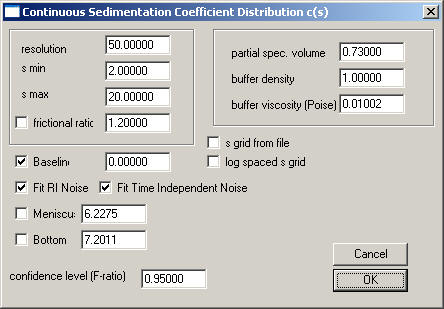
which will bring up the following parameter box with the default settings:
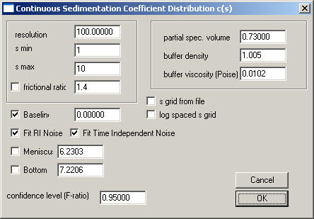
For a quick first overview, we should enter a value of 100 for the resolution parameter. For BSA, I would set s-min to 1, and s-max to 10, so that we can see both smaller fragments (if there was some proteolytic activity), as well as the oligomers which are well-known to occur with BSA. As a starting guess, a frictional ratio of 1.2 does seem reasonable for a globular protein, but BSA is somewhat asymmetric, therefore let's start with a guess of 1.4. (This will turn out to be a bad starting guess, but these settings will be refined later.) When interpreting the frictional ratio, please note that this is an anhydrous frictional ratio, and that it is only a multiplicative factor together with the solvent viscosity.
We could calculate the precise partial-specific volume of BSA, but the v-bar and the buffer density and viscosity will be completely correlated with the frictional ratio parameter (see the equations in the help-page of the c(s) model) and will only influence slightly the estimate of diffusion. (There will be no correction of s-values to s20 values.) Therefore, I suggest using an estimate of the v-bar of 0.73, and for PBS a buffer density of 1.005, and a viscosity of 0.0102.
Please note that by default all the baseline parameters are checked for interference data. We do not need to change anything there. If we were looking at absorbance data, in general the Baseline should be allowed to float (checked), whereas the Fit RI Noise and the Fit Time Independent Noise mostly would stay unchecked.
(Starting from version 8.5 and later, there's the possibility in sedfit to control the spacing of the s-values in the distribution, either logarithmically or arbitrary, but we use the default, which is linear spacing.)
After all these entries, the parameter box should look like this:
(The settings for Baseline, Fit RI noise and Fit Time Independent Noise are redundant and sedfit may automatically switch off the Baseline when RI and TI noise are used.)
If we execute the Run command (please note: this is not the Fit command, which is reserved for non-linear regression)

we will calculate the first c(s) distribution. During the calculation, we will get the information
allocating memory space...
solving Lamm equation for ... (with progress indicator)
calculating normal equations ... (with progress indicator)
regularization ... (with progress indicator)
During the last three steps, pressing the space bar on the keyboard will interrupt the calculations. This particular calculation is complete after ~ 1 min on a 700 MHz Pentium III laptop. In general, it will take longer for larger resolution, and with more scans, and it will be faster with absorbance data (and obviously it will be faster with a faster computer...).
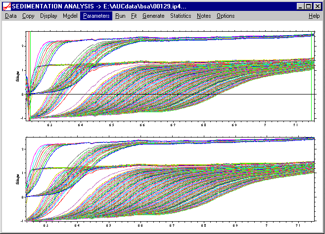
As output, fitted curves will be drawn into the data scans, the residuals are shown in a smaller plot in the middle, and a new lower plot appears showing the c(s) distribution (which at this stage is still very coarse). Also, some information will be written to the Sedfit window, which will be explained in the next paragraph.
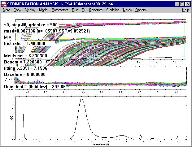
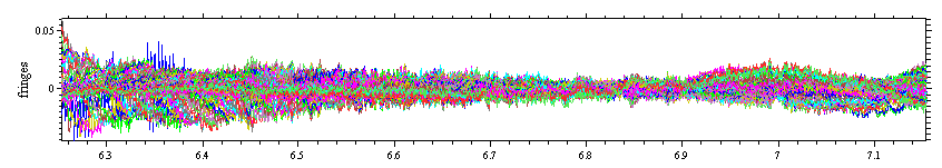
At this stage of the analysis, the most important information written to the screen is the rmsd value of 0.0074 given in the second row. (If the screen redraws, the text information disappears, but it can be retrieved by using the Display->Show Last Fit Info Again command). From the distribution, it can already be seen that most of the material sediments with s-values between 4 and 5, and that there is some larger oligomers present.
Another important aspect of the analysis at the current stage is the distribution of residuals:
Although this does not look great, yet, the absence of very large residuals at the extreme radius values indicates that the fitting limits (green lines) are OK and not too close to meniscus and bottom. A typical picture of residuals when the outer fitting limit is too close to the bottom would look like this
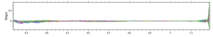
Note that the scale of the residuals plot is dominated by very large residuals at the right end of the plot. In such a case, one needs to set the outer fitting limit (green line in vicinity of the bottom) to smaller radius values. Analogously, if the residuals are dominated by very large deviations close to the meniscus, one would see this here in the left side of the residuals plot, and would need to place the inner fitting limit (green line in vicinity of the meniscus) to larger radius values.
Back to our analysis. Although the rmsd of 0.0074 seems quite good, the fit is really poor and needs to be refined before we can interpret the distribution. Without making sure that we have a good fit, artifacts can occur in the c(s) distribution (in our analysis, for example the artificial sharp peak at 7.8 S).
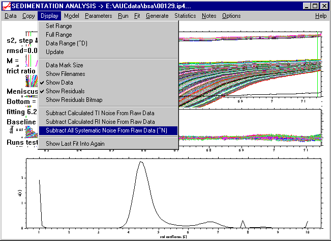
To achieve a better inspection, we can subtract the calculated systematic noise from the data with the following command (or by using the keyboard shortcut ctrl-N).
A message box will appear

that is just a reminder that we are about to modify the original data. As explained in the introduction to the systematic noise, this does not introduce any bias, as long as we keep in all the following analyses the degrees of freedom of the systematic noise, which means one should not modify the RI Noise and TI Noise in the parameter input boxes (leave them checked). As a result, we get a clear picture of the sedimentation process:

Although this fit looks already promising, it is still very coarse and must be refined in order to allow a meaningful interpretation.