back to the tutorial main page
In this example, we have followed the main steps of a c(s) analysis. These are:
1) Loading the data and getting an overview of the s-range with a coarse distribution (low resolution)
2) Refine the analysis by adjusting the s-range, and by using a higher resolution. Combine with critical inspection of the fit (e.g. using the residuals bitmap to assess systematics in the residuals)
3) Nonlinear regression of the frictional ratio parameter and the meniscus location (if necessary, slightly reduce the number of scans, and switch off the regularization for this step only)
4) Increase the resolution to final value (reload all data, and switch on the regularization again), possibly fine-adjustment of s-range. Verify that a good fit was achieved. One should generally be cautious to use a wide enough s-range, and not interpret peaks close to the extreme values of the distribution.
5) Save and export the c(s) data for plotting, storage, and further analysis.
In most cases, this allows to achieve a high resolution with baseline-resolved oligomers.
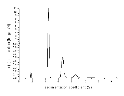
For the BSA, in the c(s) analysis we found the presence of a fraction (~1%) of small species (probably from proteolytic degradation), as well as 11-12% of dimeric BSA, 2-3% of BSA trimer, and probably a total of 0.8% of larger oligomers.

(Sharper peaks can be obtained using the Bayesian assumption that all species are pure, as shown above)
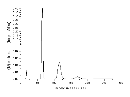
As will be shown in the following chapter, conversion to a molar mass distribution c(M) gives good estimates for the oligomer molar masses (this may not be true in general for oligomerizing systems, see the note about c(M); the SEDPHAT hybrid discrete/continuous model is the most correct and powerful way to analyze such a case):

The following chapter illustrates how the calculate a two-dimensional size-and-shape distribution c(s,M), which is free of the scale-relationship assumptions:

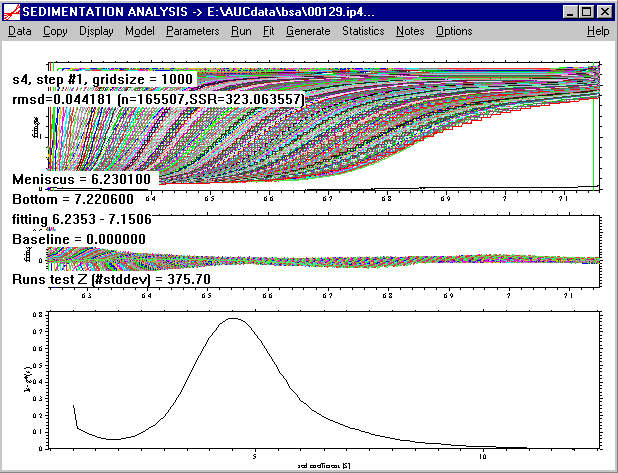
Finally, as a comparison with a g*(s) analysis, the final chapter of the tutorial will treat the ls-g*(s) analysis, which will result in the following distribution:

This is not recommended, but interesting in comparison with older methods of sedimentation analysis.