continuous distribution c(M) Lamm equation model
Model | continuous c(M) distribution
(note when not to use it, and when to use the SEDPHAT models instead)
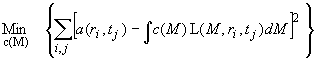
The c(M) distribution is a variant of the distribution of Lamm equation solutions:
A general introduction into the theory and practice of size-distribution analysis can be found here. By default, regularization of the distribution by the maximum entropy method is used.
It should be noted that this model is strictly correct only for mixtures of non-interacting, ideally sedimenting molecules. It can be applied to interacting molecules if the reaction is slow on the time-scale of sedimentation, or if for other reasons the species are stable during sedimentation (e.g. when working with concentrations much larger than Kd).
The result of the c(M) model is a differential molar mass distribution, scaled such that the area under the c(M) curve from M1 to M2 will give the loading concentration of macromolecules with sizes between M1 and M2.
In this particular model, the Lamm equation solutions L(M,r,t), are calculated with the approximation that all species in solution have the same weight-average frictional ratio. For each M value, using an estimate of f/f0 and values for the partial-specific volume, buffer density and viscosity, Sedfit calculates the diffusion coefficient for each M via the Stokes-Einstein formula
![]()
with R denoting the radius of a sphere with the given molar mass and partial specific volume. The sedimentation coefficient is then calculated using the Svedberg relationship
![]()
This gives the parameters s(M) and D(M) required for the Lamm equation solution. This model is described in detail in ref 1.
It is very important to note that when analyzing sedimentation velocity data, the approximation that all species have the same frictional ratio can lead to distortions in the c(M) distributions. In contrast, such distortions are in general negligible when using the c(s) distribution, and they are absent in the model for c(M) with invariant D (if the diffusion coefficient of all species is identical).
For calculating a diffusion-deconvoluted sedimentation coefficient distributions without the scaling relationships of frictional ratios, see the c(s,f) and c(s,*) models. These can transformed into a c(s,M) molar mass distribution, free of any frictional ratio assumptions.
However, there are several cases for which even this c(M) distribution is a good model:
* when f/f0 is known for all particles to be the same, such as mixtures of spherical particles (e.g. in the study of ferritin, emulsion particles, or other particles with well-known shape). In this case, a further refinement may be made if a size-dependence of the partial-specific volume is present.
* the c(M) analysis can be a good model for data of the approach-to-equilibrium, and
* it is obviously an appropriate model when analyzing sedimentation equilibrium (in this case the kernel of the distribution are sedimentation equilibrium exponentials instead of Lamm equation solutions).
* other prior knowledge can be provided, such as c(M) with a known diffusion coefficient for all species
Like with all other direct boundary models, ANY data from the entire sedimentation process can be modeled, and should be included into the analysis for optimal results. There is no need to clear the meniscus, and no need for plateaus or to exclude scans where the boundary is close to the bottom and only partially visible.
Once again: Because the molar mass scale is directly tied to the f/f0 ratio, in general the molar mass peaks in c(M) will only be correct when there is either only one main species present, or if it is known that all species have the same f/f0 ratio. Of course, it is also dependent on the correct vbar and solvent density. For samples containing irreversible oligomers (aggregates) this dependence on assumed identical frictional properties means that the apparent mass of the oligomer will in many cases not be an integer multiple of the monomer mass, and that the accuracy may not be sufficient to correctly identify the stoichiometry of the oligomer. This is true, in particular, for higher oligomers because they can deviate more from the shape of the monomer and because the relative mass error that can be tolerated for a correct identification is smaller.
In such a case, the correct way of proceeding is the SEDPHAT method for hybrid c(s) with discrete species. This will allow to enter the monomer mass as prior knowledge, and properly constrain the oligomer masses to be discrete multiples. It will give you the abundance of each oligomer (fitting their s-value). You can use the c(M) results as starting guesses. To get started with this, use the Export function of SEDFIT to transfer your data into SEDPHAT.
An alternative is the calculation of the size-and-shape distribution c(s,M).
Thus for sedimentation velocity analysis, generally the c(s) distribution and its variants are preferred over c(M), since it is the sedimentation coefficients that can be determined with high accuracy from velocity data, not molar masses.
This method should not be used in situations where the partial specific volume varies for different components (a secondary analysis to account for this may in some cases be possible), or where the frictional ratio is expected to vary widely (for example a glycoprotein where some non-glycosylated protein is also present, or a PEGylated protein with variable numbers of PEG molecules attached).
The general strategies recommended for this model are similar to those described in the tutorial on size-distribution. When using this model for the analysis of sedimentation velocity data of samples with the approximation of a uniform frictional ratio, it is recommended to treat the frictional ratio as a fitting parameter. This is described in the tutorial, and also how the c(M) distribution can be obtained after converting the c(s) distribution.
The parameters for this model are entered in the parameter input box (Parameters):
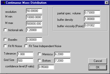
upper section specifying
the distribution range and parameters for the Lamm equation solution
middle section with experimental conditions
lower section with Lamm equation and
nonlinear regression parameters
The parameters specifying the distribution range and resolution follow the general parameter outline common to all distributions. In brief, M-min and M-max are the smallest and largest M-value of the distribution, and the resolution value determines how many M-values will be used in between. (In c(M) they are spaced non-uniform, but equidistant on a 2/3 power base.)
The frictional ratio value is the weight-average frictional ratio of all species, and if the check-box is marked, this parameter will be optimized when executing a fit command. The partial specific volume, the buffer density, and the buffer viscosity are additional parameters needed to calculate s and D for each M-value. It should be noted that Sedfit does not use this information to correct to s-values to s20,w. Also, since the Stokes-Einstein formula above shows that the frictional ratio and the viscosity are multiplicative, errors in one can be compensated in the other.
The middle section with the parameters for baseline, RI noise, and time-independent noise are the same as in all the other models (explained in detail in the non-interacting discrete species model). Also, the meaning of Tolerance, Grid Size, Meniscus and Bottom is the same as usual.
Important is the confidence level (F-ratio) setting, which determines the magnitude of the regularization. Also, the choice of the regularization method (Tikhonov-Philips 2nd derivative versus maximum entropy) is relevant, as explained in the introduction on the size-distribution analysis. This setting can be changed in the size-distribution options.
After calculating the distribution, a new plot appears in the lower part of the Sedfit window, showing the distribution. Like all distributions, it can be saved to a file (save continuous distribution), copied as graphics metafile (copy distribution plot) or data table (copy distribution table) into the clipboard. As described in the size-distribution tutorial, copying the data into another plotting program is recommended in particular if possible small contribution of species besides the main peaks are of interest. For statistical analysis (provided the fit was good, with evenly distributed residuals), the Monte-Carlo analysis can be performed.
New in version 8.7: When using the inhomogeneous solvent mode, e.g. to correct for solvent compressibility, please read the specific instructions for this Sedfit mode first. Mainly, this will mean that the s-values are corrected to standard conditions (water 20C), and that the buffer viscosity and density in this input box here also refer to standard conditions.
Please note: The calculation will be aborted if the distribution contains s-values exceeding the maximum s-value that can be observed for the given rotor speed and time of the first scan. To fix this problem, either load earlier data, or reduce the entry in the M-max field appropriately. It is recommended to stay well below this maximal value to avoid artifactual increases of the size-distribution near the maximal value.
Tips:
1) For best results, it is advisable to start with a relative small range of M-values. It is recommended to increase M-max if there is an upward curvature of the distribution at the highest M-values, and conversely, to decrease the M-min value if there is a significant contribution in the distribution at this lower M value.
2) If the Lamm equation simulations during this method are very slow, the value for changing the finite element methods should be increased (e.g. to 10).
3) In order to achieve smoother distributions, for example when studying synthetic polymers that are known to have a broad distribution, the value of P should be increased, to values close to 1 (e.g. 0.99), or even to 1.1. Also Tikhonov-Philips regularization is usually better than maximum entropy in such cases.
Reference:
P. Schuck (2000) Size distribution analysis of macromolecules by sedimentation velocity ultracentrifugation and Lamm equation modeling. Biophysical Journal 78:1606-1619