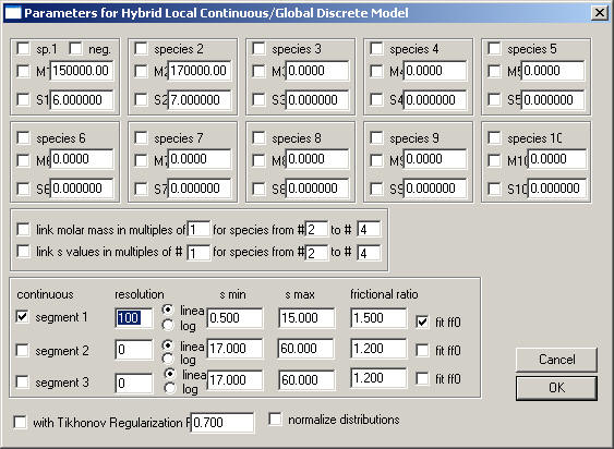
This is the most flexible model to ask questions of the type 'what species are in the mixture'. It has up to 10 discrete species which are modeled similar as the species analysis:
* the discrete species can have different amplitudes in the different experiments
* for multi-speed equilibrium experiments, mass conservation is used
* units are signal units
This is combined with continuous distributions, which are local to each experiment. The background of this model is that you can have different experiments of protein mixtures which could have different degrees of impurities (like degradation products and aggregates), and you want to focus on the discrete species that are common to all experiments.
The local distributions are similar to c(s) distributions in SedfiT, and could be regarded as an significant extension of the c(s) conformational change model, bimodal c(s) model of SedfiT or the c(s) with one discrete component.
An example of it's use can abe found in: H. Boukari, R. Nossal, D.L. Sackett, P. Schuck. (2004) Hydrodynamics of nanoscopic tubulin rings in dilute solution. Physical Review Letters (in press).
An extension for multi-signal c(s) analysis of interacting systems is available.
You can link the molar mass values: 1) switch it on with the check-box on the left; 2) enter the species # that contains the monomer molar mass; 3) enter the range of species numbers for which the entry in the mass field will be re-interpreted to mean multiples of the monomer mass. For example, if it reads: "link molar mass in multiples of #1 for species from #2 to #4" , and you have entries in the molar mass fields above of M1: 100,000, M2: 2, M3: 4, M4: 8, the molar mass values will be M1 = 100,000, M2 = 200,000, M3 = 400,000, M4 = 800,000.
Similar links can be established for the s-values.
Note, from version 4: the checkbox "neg." next to the first discrete component permits to count the signal of this component negative. This can make sense, for example, if this species is in the reference solution. For example, unmatched buffer components, such as excess salt, in the reference sector can be modeled this way. (This still requires the meniscii to match.)
This model is redundant with the multi-signal c(s) if the number of wavelengths is set to 1. The difference is that the multi-signal c(s) model allows to scale the different signals via extinction coefficients, whereas the hybrid continuous/discrete model here is in signal units.
The distributions can be integrated using the shortcut control-I, and zoomed in and out using the right mouse button. This is completely analogous to the integration and zoom functions for distributions in SEDFIT.
![]()
Examples for using this model:
1) You have oligomerization process and you're not sure of the monomer molar mass, but obviously the oligomers are in multiples of the monomer molar mass. (For a monomer-dimer system, you could constrain M2 = 2xM1).
2) You have aggregates (different extent in different experiments) you don't care about, but you need to describe them in order not to bias the analysis. Move the limits of one of the c(s) distribution so that they are outside the discrete species of interest, and cover the range of the aggregates
3) You have degradation products - use one c(s) distribution to cover the range of low s-values.
4) You have a bimodal c(s) distribution and want to optimize f/f0 separately for the different sections. You could use the bimodal c(s) model of SedfiT, but you have an extra buffer component present that you need to model.
5) you have more than 4 discrete species (set the resolution of the c(s) to zero to switch them off)
An example for the use of this model can be found in
P. Schuck. (2005) Diffusion-deconvoluted sedimentation coefficient distributions for the analysis of interacting and non-interacting protein mixtures. In: Modern Analytical Ultracentrifugation: Techniques and Methods (D.J. Scott, S.E. Harding, A.J. Rowe, Editors) The Royal Society of Chemistry, Cambridge (in press) (preprint)
![]()
You can retrieve the local concentrations and c(s) distributions via the copy command. If you copy the distribution, you will be asked
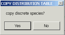
If you select YES, immediately paste it to your destination, before continuing.
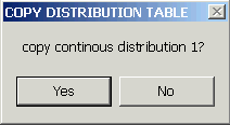
If you select YES, the previous clipboard content will be replaced by the continuous distribution segment.
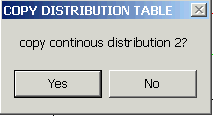
etc., which will put the corresponding section of the hybrid distribution into the clipboard for pasting into your spreadsheet software.
![]()
HINT for Using this model for equilibrium analysis: Generally, just ignore the s-values, or set them to convenient values to have a nice display (they have no meaning). When working with continuous distributions, make sure to use the option not to normalize the distribution (otherwise it'll be normalized according to the spacing of the s-vaues). You can access the M-distribution using copy and paste - you get three columns in the spreadsheet: s, M, and c.