
The principle for a single species
The limitation for multiple species
The analysis method by van Holde and Weischet (ref 1) is a graphical extrapolation method for deconvoluting diffusion in sedimentation boundaries. The strength of this method is that it is fast and allows easily to diagnose qualitatively different types of sedimentation processes (ref 2).
The basic idea is that diffusion proceeds on a square-root of time scale, while sedimentation is linear in time. In theory, after infinite time, all species with different s-values will be separated. In practice, the data analysis starts with a graphical inversion of different parts of the sedimentation boundary (boundary fractions), which is combined with an extrapolation to infinite time on a 1/sqrt(time) scale. This gives an integral sedimentation coefficient distribution G(s) which reflects the relative amounts of species sedimenting with different s-values. Although there are practical and theoretical limits in the resolution of heterogeneous mixtures of small or intermediate-sized molecules, it is an elegant approach to extract qualitative information on the sedimentation process, because the graphical extrapolation allows to compare the sedimentation velocity of different parts of the boundary. The presence of non-ideal concentration dependent sedimentation and heterogeneity can be diagnosed this way.
On the other hand, such a diagnosis can also be made in a more quantitative way, though with more computation time, by using direct boundary models for non-ideal sedimentation or size-distributions c(s) (ref 3 and ref 4). In particular for the analysis of non-interacting heterogeneous mixtures including small to medium sized species, the c(s) method has shown higher resolution and sensitivity.
Because of the graphical inversion of the sedimentation boundary required, this method cannot be applied to interference optical data where the observed data are only obtained in superposition with systematic noise. In order to overcome this limitation, one can exploit the equivalence between boundary fractions and area fractions of ls-g*(s). By analyzing different sets of sedimentation boundaries with ls-g*(s), which can take into account systematic noise, one can arrive at boundary divisions from interference optical data, which can then be extrapolated to infinite time with the usual van Holde-Weischet scheme (see extrapolation of ls-g*(s) to infinite time, ref 3). Better results are obtained, however, by using a c(s) analysis.
In the following, the principle is described in more detail, followed by the boundary diagnosis, and a description of the limitations for heterogeneous mixtures that do not show clearly separated sedimentation boundaries.
The principle for a single species
In brief, the basis of the method is the Faxén approximation of the Lamm equation, which can be written as
(1)

with the meniscus position rm, the boundary position of a non-diffusing species r*(t)=rmexp(w2st) and the error function F. It has a first term describing radial dilution, a second term (1-F) for the diffusional spreading, and the movement of r*(t) describes the boundary movement. If we scale each individual scan from 0 to 100% (100% corresponding to the plateau of each scan), we can ignore the effects of radial dilution, and we deal only with the fractional plateau concentration:
(2)

Although this transition to fractional plateau values simplifies the theory, on the experimental side this requires us to establish both the solvent and the solution plateau for each scan (see below). If we divide the boundary in N fractions (i.e. divide the plateau concentration into N concentrations ci = icp/N), we can measure the radial position Ri at which any of these fractional plateau concentration ci are observed. Each of these radial positions Ri can then be transformed to an apparent sedimentation coefficient according to s*app,i = ln(Ri/rm)/w2t. With Eq. 2 we can predict where this fractional concentration ci should occur:
(3)

This equation can be inverted, by using the inverse error function F-1:
(4)

The key of Eq. 4 is that s*app,i of each fraction is equal to the true sedimentation coefficient of the species plus an extra contribution from the diffusion term. This extra contribution depends on the fraction of the boundary: For example, for the molecules in the leading edge of the sedimentation boundary diffusion was mainly in the same direction of the sedimentation, while in the trailing end of the boundary, diffusion occurred mainly in the opposite direction.
Knowing that for a single species (in the Faxén approximation) the s*app,i of each fraction should behave this way, we can analyze our data by determining graphically the s*app,i values of each fraction, and then fitting the time-course of the s*app,i (t) with a straight line on a 1/sqrt(t) scale.
This procedure is illustrated here (simulated data for a single species with 10 S):

We divide the sedimentation boundaries in fractions (here visible in the 10 vertical steps), and convert these to apparent sedimentation coefficients s*app,i values of each fraction.
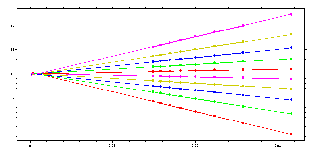
The s*app,i values for each fraction are shown here in a different color, and the straight lines are the best-fit straight line on the 1/sqrt(t) scale. If we plot the s-value that we obtain in this extrapolation to infinite time (zero intercept in the above curve) as a function of boundary fraction, we get the integral sedimentation coefficient distribution:

Please note the scale of this graph (9.92 to 10.08) -- this is essentially a vertical line with a precision of approximately 0.5%

The use of the G(s) analysis for boundary diagnosis is described in ref 1 and ref 2. Empirically, we can observe that if there is (repulsive) concentration-dependent sedimentation, the upper part of the boundary sediments slower than predicted for an ideal species, and we get the following extrapolation picture:
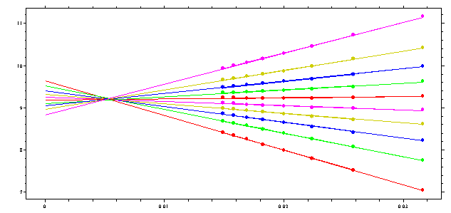
(the sedimentation data were the same as for the ideal species above, but using finite element Lamm equation solutions simulated for non-ideal concentration dependent sedimentation with repulsive interactions, with a coefficient ks = 0.1).
On the other hand, if the upper part of the boundary sediments faster, because of heterogeneity or attractive interactions between species, we get
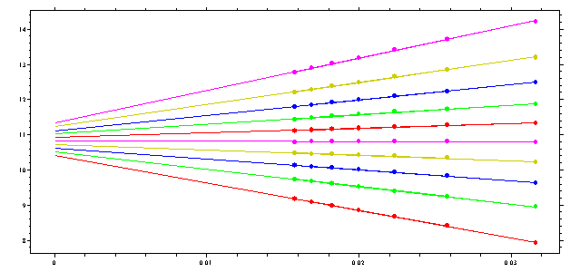
(this is based on the same simulation as above, but simulating attractive interactions).
It is clear that this picture of the nonlinear regression has diagnostic value: if the lines cross at zero, the sedimentation is ideal, if they cross to the right there is repulsive non-ideality, if they have an imaginary cross point left of the zero, it indicates either heterogeneity of ideal species or attractive interactions between the macromolecules (attractive non-ideality). This diagnostics can also be made from the G(s) curves obtained:

with the repulsive case in red, the ideal in black, and the attractive (or heterogeneous) case in blue.
Again, this diagnosis can also be made by direct boundary modeling and comparison of the data and the fit with different models. This may not be as fast and convenient as the van Holde-Weischet method, but it can be interpreted quantitatively.
The limitation for multiple species
Let's consider a mixture of two ideally sedimenting species. Following the scheme above, we can describe this situation by the sum of two Faxén approximations
(5) 
We can write this formally equivalent to Eq. 2:
(6)
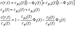
which shows that the fractional plateau concentration is now dependent on two instead of one error function. The ratio of the two will be slightly time-dependent (because of the faster radial dilution of the faster sedimenting species), and we can abbreviate the fractional plateau concentrations as a1 and a2.
(7)
![]()
For our boundary divisions analogous to Eq. 3, we get
(8)

If we try to invert the error function, we get stuck at this point:
(9)

The problem is that the simple inversion of the error function is not possible any more. This inversion gives only the simple result expected in case either one of the error function terms is negligible. In practice, this means that only boundary divisions give a true s-value that originate from positions in the solution where the sample is homogeneous! This is fulfilled at infinite time, when all species with different s-values have separated, but this is not fulfilled for many real experiments with small solutes (large diffusion), finite solution columns, and finite observation times.
What is the consequence of that? Let us consider the sedimentation profiles of two species with 5S and 7S at equal concentration at 50,000 rpm. If we assume a diffusion coefficient of 3x10⁻⁷cm2/sec for both, we get the following boundaries:
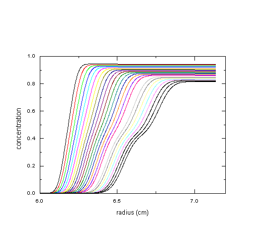
If we apply the van Holde-Weischet analysis to this data, we get the following:
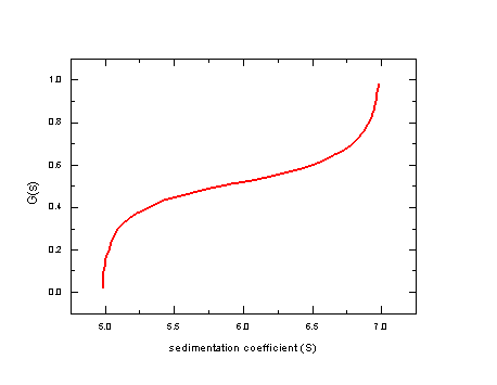
Instead of one piecewise vertical line with one section at 5S and one at 7S, we get a continuous transition of s-values. The extreme values are correct at 5S and 7S, because the lowest and the highest part of the boundary represent nearly pure material. In the intermediate, however, we have a mixture, and because the inversion of the error function breaks down in this case, we only get an intermediate value that cannot be quantitatively interpreted.
This effect is strongly dependent on the relative magnitude of the difference in the sedimentation coefficient and the diffusion coefficient: If we assume a diffusion coefficient of only 1x10⁻⁷cm2/sec, the sedimentation boundaries are visually separated, and the G(s) approaches the ideal of two vertical sections (green line). On the other hand, if the diffusion coefficient is 10x10-7cm2/sec, no separation is visible at all, and we get the blue line, which contains only limited information.
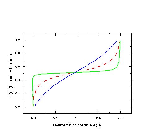
We find that the G(s) method can deconvolute the effects of diffusion, but only for well-separated species. Heterogeneity can be diagnosed, but diffusion cannot be taken into account at the same time (except for very small ratio of D/s, i.e. large species). In theory, with infinite long solution columns, this limitation could be overcome, but not under experimentally practical conditions.
It should be noted, however, that in contrast to the G(s) method the c(s) method can still identify the two species, even in the worst-case scenario shown here (the blue line):
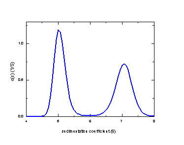
Due to the maximum entropy regularization used, the difficulty of resolving the species translates into in relatively broader peaks. However, they are clearly baseline-separated and the area under the peaks can be analyzed quantitatively (here with area ratios of 53% and 47%, respectively).
There are three main reasons for the ability of c(s) to resolve species where G(s) fails: 1) the theoretical difficulty of G(s) in the inversion of multiple error functions; 2) the much larger data set that can be analyzed with c(s) as compared to G(s) (in c(s) the data are not constrained to the scans where meniscus or solution plateaus are established); 3) the neglect of information on the plateau heights in G(s). These issues are discussed in more detail in ref 3.
The implementation in SEDFIT is described in ref 3 and ref 4. Briefly, the plateau is determined from the average signal in the 0.05 cm next to the right fitting limit. The solvent plateau is determined by the average signal of the last scan in the 0.05 cm next to the left fitting limit. The boundary is then divided in N fractions, with concentration increment dh. The radial positions of the boundary fractions is determined as the mean value of all data within 0.5xdh of the concentration ci: Ri = mean {r, with dh(i-0.5)< c(r) < dh(i+0.5)}. This method of calculating the position of the boundary fraction is designed for a high number of fractions, where the boundary increment dh for each fraction are comparable in size to the noise of the data, and it extracts the boundary positions in a least-square sense, not requiring smoothing of the data. Because of the error introduced from the data in the plateau region, the first and last boundary fraction are excluded. In the least-squares algorithm implemented in SEDFIT, it is ensured that all boundary fractions in all scans have at least one data point, otherwise the number of boundary fractions N is automatically reduced. This is followed by the calculation of the apparent sedimentation coefficients s*app,i = ln(Ri/rm)/w2t, and linear regression according to Eq. 4.
In addition to the plot of boundary fraction extrapolation and the distribution G(s), SEDFIT also calculates from the linear regression Eq. 4 the best-fit sapp values for each boundary fraction. This is then converted into a series of step-functions (similar as those in the ls-g*(s) method), which are displayed with the raw data, and residuals can be assessed. Although the van-Holde-Weischet method is not a direct boundary model, the representation of the 'best-fit' boundary fractions in comparison with the original data still displays which features of the original data are well-described, or which features were neglected.
The differential apparent sedimentation coefficient distribution can be used to define boundary fractions. This is apparent from the fact that it is derived from modeling the data by superpositions of step-functions (see the ls-g*(s) tutorial). Therefore, the same extrapolation can be used for the s*app,i values derived from area fractions of ls-g*(s) as for the s*app,i values derived from division of the sedimentation boundary. The advantage of the ls-g*(s) extrapolation is that this is applicable to interference optical data.
Because the same fundamental limitations apply to the ls-g*(s) extrapolation as described above, this model is included in SEDFIT mainly for methodological exploration. For a detailed data analysis, I would recommend in most cases the c(s) analysis.
This extrapolation of ls-g*(s) to infinite time is implemented in the following way: The total set of scans used for analysis is subdivided in sequential sets of scans, each taken at a time interval centered at ti . For each set, a differential sedimentation coefficient distribution ls-g*(s)i is calculated, and divided into N equal area fractions Aj. The s-value sij(Aj) at which the area under ls-g*(s)i equals Aj corresponds to the s*app,i values defined in the vHW method via the boundary position. It should be noted that the area under the ls-g*(s) curves corresponds to the loading concentration (Eq. 4), and therefore, these fractional areas are equivalent to boundary fractions, and the average sedimentation coefficient sij in a given area fraction at time ti directly corresponds to the s-values calculated for each boundary fractions in the van-Holde Weischet method. As a consequence, the same extrapolation procedure can be applied.
Details of the theory and practical application of this method are described in Ref 3.
References
(1) K.E. van Holde and W.O. Weischet. (1978) Boundary analysis of sedimentation velocity experiments with monodisperse and paucidisperse solutes. Biopolymers 17:1387-1403
(2) B. Demeler, H. Saber, J.C. Hansen. (1997) Identification and interpretation of complexity in sedimentation velocity boundaries. Biophys. J. 72:397-407
(3) P. Schuck, M.S. Perugini, N.R. Gonzales, G.J. Howlett, and D. Schubert. (2002) Size-distribution analysis of proteins by analytical ultracentrifugation: strategies and application to model systems Biophysical Journal 82:1096-1111
(4) P. Schuck (2000) Size distribution analysis of macromolecules by sedimentation velocity ultracentrifugation and Lamm equation modeling. Biophysical Journal 78:1606-1619.