Introduction to g*(s) analysis
The definition of ls-g*(s) and the solution of the integral equation
Equivalence of ls-g*(s) and g(s*)
Introduction to g*(s) analysis
The g*(s) analysis has been very popular over the last several years in the form of a data transform derived from dcdt. One of the virtues of this method (as opposed to the calculation of g*(s) from the radial derivative dc/dr) is that the time-difference dc/dt eliminates the time-invariant noise usually encountered in interference optical data. One difficulty in practice is that dcdt is approximated by Dc/Dt, which imposes the well-known constraints on the number of scans, steepness of the sedimentation boundary analyzed, and the magnitude of the displacements between scans, and which can even lead to distortions of the distribution for small molecular weights. With the development of systematic noise decomposition we can calculate the same g*(s) distribution differently, in the form of a direct boundary model and using least-squares principles. This will be described in the following, and it will be shown below that this approach eliminates some of the constraints.
The distribution is termed ls-g*(s) to indicate the least-squares basis of the analysis. In contrast to the dcdt strategy, there is no transformation of the radial variable into a s*, therefore we call it ls-g*(s) instead of g(s*). The star in g*(s) indicates that it is an apparent sedimentation coefficient distribution, meaning that diffusion is not taken into account. This is certainly a good model for very large molecules when diffusion is negligible on the time-scale of the velocity experiment. For smaller molecules, diffusion can be taken into account by using the c(s) method, but this is not done in the ls-g*(s) approach. As a consequence, the sedimentation coefficient distribution is broadened by diffusion.
Diffusional broadening can, in principle, be analyzed at a later stage by fitting Gaussians to the g*(s) distribution. However, this is not always very precise, as the Gaussians are based on the Faxén approximation of the Lamm equation (see the discussion in ref 1). For quantitative analysis, more precise is modeling of the original sedimentation data on the basis of numerical Lamm equation solutions (for example, using the independent species model of Sedfit), or modeling dc/dt using the approximate analytical solutions of the Lamm equation (e.g. with John Philo's software (ref 4)). However, in my view, the strength of the apparent sedimentation coefficient distribution is not so much the quantitative analysis, but that it can be very descriptive.
If we understand the g*(s) distribution as a data transformation (this attribute can be assigned with equal justification to the g(s*) and the ls-g*(s) distribution), then we can apply it in a descriptive sense to any sedimentation data, even if there are chemical reactions or other concentration-dependent sedimentation processes. Comparison of the g*(s) distributions from different experiments at different loading concentrations can give some information about the underlying processes.
Sometimes, the g*(s) distribution is considered to be a 'model-free' representation of the sedimentation data. It is very important to keep in mind, however, that g*(s) is based on a specific model - that of non-diffusing particles. In fact, this model is in most cases very poor. If we compare it with the c(s) distribution, where we use the model that all molecules have the same weight-average frictional ratio, g*(s) would be equivalent with the assumption of all species having an infinite frictional ratio (and in fact, the results of c(s) with f/f0 = 10 and ls-g*(s) are very similar). This is not very realistic, and this is the reason for the much lower resolution of g*(s) as compared to c(s). However, in some cases the sedimentation process is very complex (e.g. non-ideal concentration dependent sedimentation or complex heterogeneous chemical reactions), and currently, diffusion can not be taken into account properly. This is where the model of non-diffusing particles and g*(s) is highly useful. Obviously, it is also the appropriate model if diffusion can be neglected (such as for very large particles).
Note the new feature introduced in version 8.7 of Sedfit which allows to use the framework of the ls-g*(s) to generate a back-transform of the g(s*) distribution [from dc/dt] into the original data space. This eliminates the drawback of the g(s*) by dc/dt transform of not providing any control over how well the original data are represented.
The definition of ls-g*(s) and the solution of the integral equation
The apparent sedimentation coefficient distribution g*(s) can be defined as the differential distribution of non-diffusing species
(1)
![]()
where c(r,t) is the measured sedimentation profile, and U(s,r,t) is the sedimentation profile of a non-diffusing species:
(2)

Bridgman has shown how to calculate g*(s) from the radial derivative dc/dr (ref 2), and Stafford has described the calculation of g*(s) from the time-derivative dc/dt (ref 3). Sedfit uses a different approach - the direct solution of the integral equation (Eq. 1) (ref 1).
This can be done by discretization of Eq. 1, very similar to the approach described in the introduction to the size-distribution analysis. We approximate Eq. 1 by
(3)

which can be solved as a least-squares problem:
(4)

(where the summation over r and t is over all experimental data points). The coefficients g*i(si) represent a discretized approximation of the size-distribution g*(s). As shown in the general case, we can introduce additional terms for the description of the systematic noise, including the time-invariant noise as well as jitter and integral fringe shifts.
One technical difficulty in the discretization of the integral equation Eq. 1 is the choice of the grid of s-values si. As described in the introduction to regularization, too fine discretization can lead to high artificial oscillations, while too coarse discretization may not provide sufficient detail. Therefore, regularization is used, and a penalty term for oscillations is added to the minimization problem:
(5)

The second term serves to stabilize the solution by Tikhonov-Phillips regularization, and like the maximum entropy regularization, it is adjusted to give the most parsimonious solution within a predefined confidence limit (see the introduction to size-distributions, regularization, and the paragraph on the difference between regularization and smoothing).
The important property of Eqs. 4 and 5 is that they are linear. Therefore, we can easily calculate the distribution g*i(si), as there exists a unambiguous minimum that can be calculated directly by well-known algebraic methods. Because of the 1:1-relationship between the data and the g*i(si) distribution, this can be considered a 'data transformation'. Similar to the other size-distributions, Eq. 5 is solved by normal equations, using Cholesky decomposition and a variant of the dual-vector method NNLS by Lawson and Hanson for excluding negative values for g*i (more information can be found here).
The analysis in Sedfit requires some user input about the discretization, i.e. resolution, s-min, s-max, and the confidence level, these are common to all size-distributions and described here.
The meaning of the definition of ls-g*(s) in Eq. 1 and the discretization Eq. 3 can be visualized in the following way: The sedimentation profiles U(s,r,t) are series of step-functions, describing the evolution of an infinitely sharp boundary with radial dilution:

The different U(si,r,t) describe families of such step-functions with different sedimentation rate si. In essence, calculating g*(s) according to Eq. 3 is asking the question of what superposition of step-functions can be found that describes the data c(r,t) best. This is illustrated here:

In gray are sedimentation profiles c(r,t) (here simulated sedimentation profiles of a single species with added noise), and in blue is shown the best-fit discretization into step-functions. It is obvious that we need smaller steps with lower sedimentation rate (green), larger steps with intermediate sedimentation rate (red), and small steps again with high sedimentation rate (black), in order to describe the data well. The magnitude of the steps plotted as a function of the sedimentation rate

is identical to the apparent sedimentation coefficient distribution ls-g*(s).
Equivalence of ls-g*(s) and g(s*)
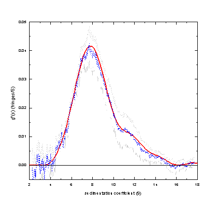
The distribution ls-g*(s) is equivalent to the distribution g(s*) derived from dcdt, because both distributions are based on an equivalent definition of g*(s) as the distribution of non-diffusing particles. If we apply both methods to the same data set

we get essentially the same results from dcdt (dashed blue, with confidence bands in gray) and ls-g*(s) (red):

New: We also can take the results from dcdt, build up a boundary model with step-functions as in ls-g*(s), determine the best-fit TI noise, and compare this with the original data - this represents a back-transform of dcdt (see Analytical Biochemistry 320:104-124).
For the same sedimentation data shown above, ls-g*(s) allows to incorporate a much larger time-interval without compromising the resolution:

NOTE: The time-interval should not be so large that the quality of fit decreases. This is true, in particular, for boundary shape analysis and when interpreting details of the distribution. For example, for moderately-sized proteins < 100 kDa, this usually leads to a time-interval approximately 2 - 3 fold that recommended in DCDT+. However, this is purely dependent on the extent of diffusion, which means that a larger rotor speed can increase the permissible range of boundary displacement. Also, the permissible time-interval increases with larger species.
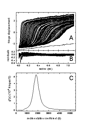
Another example is from the analysis of a dispersion:

Here, the model of no diffusion is a very good approximation, and we get a good fit. The size-distribution is very broad. Nevertheless, it is well-defined and does not suffer from a dependence on the choice of the data subset. More information about this example, and the comparison with the results from dcdt are given in ref 1.
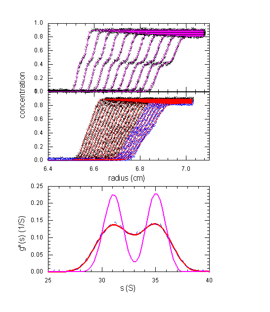
The following shows large boundary displacement as it might occur in an absorbance experiment with two species with 31 and 35 S, at 50,000 rpm (top) and 30,000 rpm (middle).

The fit of the 50,000 rpm data by ls-g*(s) (magenta) gives two well-separated peaks. However, because of the large boundary displacement, we cannot analyze the 50,000 rpm data with dcdt. This is possible if we run the same experiment at a lower speed and take a data subset (blue circles). This gives a g(s*) from dcdt as shown in the lower figure as blue dotted line, which is essentially identical with the results of ls-g*(s) of the same data, or the complete data shown at this speed. However, it is clear that the ability to run species at higher speeds does produce much better separation, and as a consequence, resolution in ls-g*(s).
On boundary shape analysis in g*(s)
Historically, the quantitative analysis of g*(s) profiles by Gaussian fitting has been used to determine the diffusion coefficient D and therefore the molar mass M of a species. This approach is outdated, because it is based on relatively simple analytical approximation of the Lamm equation, where now more precise solutions are available.
The optimal procedure within the Sedfit/Sedphat package for determining the molar mass of a species is the use of the hybrid discrete/continuous distribution in Sedphat, which models the species of interest with a discrete finite element Lamm equation solution, and allows for other species to be modeled by continuous segments. This is more precise than the molar mass values from the c(M) distribution, because the latter is based on a weight-average f/f0, where the weight-average may be biased by other species in the sample. However, a c(s) or c(M) distribution is usually extremely helpful because it can take advantage of the data from the complete run and - due to the deconvolution of diffusion - reveal if there is heterogeneity within the diffusion-broadened boundary. Unrecognized heterogeneity would lead to artificially low molar mass estimates.
Background: The analysis of boundary spreading can be based on the Faxén solution of the Lamm equation, which can be written approximately as
(5)

with the meniscus position rm, the boundary position of a non-diffusing species r*(t)=rmexp(w2st) and the error function F. It has a first term describing radial dilution, a second term (1-F) for the diffusional spreading, and the movement of r*(t) describes the boundary movement. The radial derivative can be expressed as a Gaussian
(6)

If we use the picture of non-diffusing species where at a given time each radius position corresponds to a particular s-value, we can use the transformation
(7)
![]()
to express the radial profile of dc/dr in the space of apparent sedimentation coefficients, leading to
(8)

, i.e. the diffusional spread translates into a Gaussian distribution of apparent sedimentation coefficients.
How does this apply to ls-g*(s)? As indicated in Eq. 1 and 2 above, ls-g*(s) is defined as
(9)
![]()
with
(10)

Taking the radial derivative, we get
(11)

where the derivative of the Heaviside function turns into the Dirac delta-function:
(12)

and in combination with (11) and (8) we arrive at
(13)
![]()
which means g*(s) is a Gaussian distribution.
In summary, this shows that the definition of ls-g*(s) faithfully represents the radial derivative of the concentration distribution, which leads to a Gaussian distribution for a single diffusion species in the approximation of the Faxén solution of the Lamm equation.
From theory to practice: The preceding derivation was for a single point in time, i.e. for a single scan. Although one could in principle calculate such a ls-g*(s) distribution from a single scan, this is not implemented in Sedfit, as it would not allow to distinguish systematic signal offsets from the interference offsets, and exhibit poor signal-to-noise characteristics.
For more than one scan, the resulting g*(s) distribution represents something like an average of Gaussians for the individual scans, which one can expect to lead to deformations of the Gaussian, and the problem of determining the correct time-point for evaluating the diffusion constant in Eq. 13. As a 'naive' assumption, which I would favor, one could take the average time-point of the scans considered, but it has not been shown that this is indeed correct. (This problematics exists in similar form also for the DCDT approach, which also relies on at least two scans taken at different points in time, but the point of averaging appears in a different space.) Although it follows that any deviation from a single scan or infinitesimal time-range is problematic, it should be noted that even then there are errors resulting from the underlying Faxén approximation of the Lamm equation.
A handle to this problem can be obtained from considering the quality of fit of the ls-g*(s) model to the raw data. If the residuals are random within the noise of the signal, it could be argued that the time-points of any of the scans is just as good as another. Although the particular choice would lead to different D values, this should be understood as a translation of the noise in the signal into the range of D values. The requirement for a good fit excludes large time-intervals for data where the diffusional fluxes are high (in particular, for small molecules and low rotor speeds). If, on the other hand, diffusional fluxes are small and a correspondingly larger time-interval can be chosen without compromising the quality of the fit (translating to a larger relative range of D-values), this would satisfy our expectation that in experiments with high s and low D the diffusion constant is not very well determined.
For boundary shape analysis by secondary modeling of ls-g*(s), therefore, it is essential that the fit is of good quality. This is just a reflection of the fact that if the fit of a model is not good, not a lot of trust can be placed in the details of the parameters obtained. For small species and low rotor speeds (i.e. at high diffusional fluxes) this requires smaller time-intervals than larger species or higher rotor speeds.
As outlined above, I would strongly recommend the use of more precise Lamm equation solutions for analyzing the molar mass.
In brief, this model describes the sedimentation of a distribution of non-diffusing species. It is closely related to the results of g(s*) by dcdt, but in the form of a direct boundary model. When applied to a data set where the dcdt method is applicable (i.e. a not too much boundary displacement and a limited number of scans), ls-g*(s) and g(s*) by dcdt give the same results. However, ls-g*(s) has several advantages that make it more versatile:
1) As a direct boundary model, there is no differentiation step and no approximation of dc/dt by Dc/Dt. As a consequence, we do not need to take data from small time-intervals only. There is no artificial broadening caused by having too many scans! (A mathematical analysis of the broadening that occurs due to the approximation of dc/dt by Dc/Dt is included as an appendix to ref 1.) Limitations are imposed by the requirement to have a good fit of the data.
2) Ability to work with scans that have large displacement is highly useful when analyzing absorbance data, but the method works equally well for interference data, where systematic noise decomposition is used.
3) Because large boundary displacement is not an issue, experiments can be run at higher rotor speeds, which can translate to higher resolution.
4) It is suitable for combination with non-linear regression, for example for determining the exact meniscus position.
The practical use of the method is described as a chapter of the step-by-step tutorial on size distributions, and can also be seen in the example of using Sedfit.
When working with interference optical data (or other data requiring time-invariant noise analysis), the method works best with large data sets, and with data where the boundary has cleared the meniscus. This minimizes a fundamental problem of correlation of small s-values of the distribution with the degrees of freedom from the unknown time-invariant noise.
References
1. P. Schuck and P. Rossmanith (2000) Determination of the sedimentation coefficient distribution g*(s) by least-squares boundary modeling. Biopolymers 54:328-341.
2. W.B. Bridgman (1942) J. Am. Chem. Soc. 64:2349-2356
3. W.F. Stafford (1992) Anal. Biochem. 203:295-301
4. J.S. Philo (2000) A method for directly fitting the time-derivative of sedimentation velocity data and an alternative algorithm for calculating sedimentation coefficient distribution functions. Anal. Biochem. 279:151-163