This data type is for an experiment where one measures steady-state binding of a soluble molecule to surface-immobilized sites. The concentration of the soluble molecule is held constant, for example, by virtue of a flow system. These data can be derived, for example, from a Biacore SPR instrument.
For a 1:1 interaction, the concentration-dependence of the fractional saturation of the surface sites follows a Langmuir isotherm. More complex models are available, as well, and are planned to be implemented in the future. When using the parameter boxes, by convention, the immobilized molecule is the binding partner "A".
For using this model, one needs first to generate an ASCII text-file with the following format:
SignalImmobA ConcB1 Signal1
SignalImmobA ConcB2 Signal2
SignalImmobA ConcB3 Signal3
SignalImmobA ConcB4 Signal4
SignalImmobA ConcB5 Signal5
...
where "SignalImmobA" refers to the surface concentration of the immobilized molecule in arbitrary units (such as RU). Note that the surface concentration of A can later be treated as a fitting parameter. Also, it will be the same for each line. "ConcB1", "ConcB2", etc. are the concentrations of the soluble binding partner, in micromolar units. "Signal1", "Signal2", ... refers to the measured steady-state surface binding value in the same units as "SignalImmobA" (such as RU).
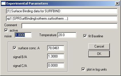
The default extension is "*.surfisotherm". For loading this data, use the function "Data->Load New Surface Binding Equilibrium Data (Flow)". A file selection box will appear that lets you select the *.surfisotherm file with the raw data. After that, the Surface Binding parameter box pops up:
The data-type specific parameters to be entered are:
surface conc. A: This is the signal of immobilized active A. For example, this can be the difference in signal in RU before and after immobilization. The value shown here will be the value "SignalImmobA" used in the file.
signal B/A and signal C/A: It is possible to account for the fact that the soluble analyte B (or C) have different signal contributions, for example, due to differences in molar mass. In this case, set signal B/A to the ratio Mw(B)/Mw(A).
When done, press "OK", and then save the data as xp-file with the function Data->Save Experiment.
The data analysis proceeds as in other data analysis, with the selection of the model, the estimation of starting parameters, the Run and the Fit command. You can save the analysis in a configuration file.
Note, the data will be independent on things like s-values, enthalpies, concentration parameters, rate constants, etc. Please don't float these parameters during the fit.