The data menu provides the main functions to generate, save, load, and remove experimental data files (or data channels). For the general concepts on how to use the experiments, see this getting started page.
You must first generate an experiment file before you can load it. This can be done using the function "Load New...", followed by input of the necessary parameters (entering the parameters in Experimental Parameters, and graphically as described in detail in SedfiT help), and then saving them as 'xp-files'.
Load New ... Data: Sedimentation Velocity, Sedimentation Equilibrium, Multi-Speed Equilibrium, DLS, Isotherm, ITC, Surface Binding Isotherm
set current configuration as startup default
copy all data and save as new config
This allows you to load a previously saved 'xp-file' and include it in the global analysis. Once you've generated an 'xp-file', you will not need to specify each time the data filenames, meniscus, bottom, fitting limits, baseline requirements, extinction coefficients, buffer conditions, etc. This is all automatically loaded. See Experiments for details.
keyboard shortcut is control-E.
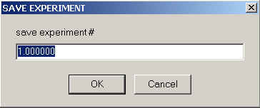
This will save the current experimental parameters of a specific experiment to a file (under a new filename). This will include the parameters in the Experimental Parameters box, and some of the local concentration or molar ratio parameters.
The particular experiment is selected according to it's experiment number (same order as the display, left to right).
What is not saved are links describing the sharing of local parameters. They need to be manually re-established (and they are obviously dependent on experiment number, i.e. order of loading the experiments).
This is a convenient command to save the current status of all loaded experiments to their respective files. Note that this only updating the files, which means it will overwrite older parameters contained in the xp-files. If this is not desired, you can use the previous "Save Experiment" command and specify new filenames.
keyboard shortcut is control-A
This function will remove a specific experiment (referred to by experiment number) from the global analysis. For only temporarily removing an experiment from consideration in a global fit, but without removing it from the SedPHaT memory, you can use the 'active' checkbox to inactivate an experiment. Alternatively, if you just want to execute a Run or Fit command for a single experiment, you can do that with the 'Single Experiment Run' or 'Single Experiment Fit' functions.
![]()
This family of functions have the purpose to load raw data files, request appropriate ancillary experimental information, and to generate a complete Experiment in the memory of SEDPHAT, which can be saved as an xp-file (by default the user will be prompted to enter a filename for the associated xp-file). This xp-file is what in the future will be loaded (using the Load Experiment function), instead of the raw data. In this way, we don't have to enter the ancillary information twice.
The Load New... functions are automatically invoked when using drag-and-drop of certain raw data files (like *.dat for ITC, *.isotherm for isotherms, *.dlsdat for DLS data, and *.surfisotherm for surface binding isotherms).
These functions are specific to the different data types:
This is data from a single centrifuge cell comprising the time-course of sedimentation. This sedimentation velocity data is loaded just as in SedfiT. For more detailed instructions, see the SedfiT help web. After selecting the data, an experiment box will appear and information needs to be supplied. For details, see the Sedimentation Velocity Box.
This function loads a single sedimentation equilibrium profile and makes it into an experiment. Obviously, you should only select a single file when using this function. Global analysis will be accomplished by loading many such sedimentation equilibrium experiments, i.e. executing this command many times, each time generating a new data channel. After selecting the data, an experiment box will appear and information needs to be supplied. For details, see the Sedimentation Equilibrium Box.
This allows to load several sedimentation equilibrium profiles at once into a combined experiment (data channel). They have to be from the same cell, be acquiring with the same signal (i.e. same wavelength or all interference data), but be at different rotor speeds. The advantage of loading such files together is that they can be conveniently prescribed to have a common baseline (or radial baseline profiles). They also automatically have the same meniscus, bottom, extinction coefficient, and loading concentration. Although the latter parameters could be defined to be shared, setting multiple scans at different rotor speeds up as a multi-speed sedimentation equilibrium experiment is more straightforward.
Note: Multi-speed equilibrium data sets can have disadvantages when mass conservation is not used and concentration parameters are to be shared. In this case, the concentration parameters are shared between pairs of files (1st in exp. #1 with 1st in exp. #2, 2nd in exp. #1 with 2nd in exp. #2, etc.). Therefore, two multi-speed equilibrium experiments without mass conservation but with shared concentrations have to be equivalent in the number and sequence of loaded scans. Because of these complications, sharing in this situation is currently not enabled between multi-speed equilibrium experiments.
For more details on the implications of multi-speed sedimentation equilibrium baseline parameters, see the parameters introduction and the examples.
After selecting the data, an experiment box will appear and information needs to be supplied. For details, see the Multi-Speed Equilibrium Box.
This loads an autocorrelation function from dynamic light scattering into an experiment channel. The format is a 'dlsdat-file' as generated by SedfiT. Therefore, you have to use SedfiT first, use the function "Options->Loading Options->Import DLS Data" of SedfiT, and save the data (which is automatically done in the 'dlsdat' format). SedfiT allows you to read raw autocorrelation data files exported in a variety of formats from Brookhaven Instruments, Protein Solutions, and ALV.
After selecting the data, an experiment box will appear and information needs to be supplied. For details, see the DLS Data Box.
For an overview of SV isotherm analysis, see this page.
This function allows to load an ASCII (ANSI) txt file (tab delimited) containing isotherm data of weight-average sedimentation coefficients as a function of concentration (sw(c)), or weight-average molar mass values (Mw(c)) as a function of concentration.
For more detailed analysis of rapid interacting systems, isotherms are available for the s-value of the fast component of the reaction boundary and for the amplitudes of the undisturbed and the reaction boundary component of the asymptotic boundary based on Gilbert-Jenkins theory. The amplitudes and weight-average s-values of the reaction boundary can be obtained from integration of the c(s) profiles in SedfiT.
For slowly interacting systems, isotherms for the partial populations of the different species are available. These also are apparent from integration of the c(s) profiles in SedfiT.
Isotherm analysis is only implemented for interacting models, i.e. self-association and hetero-association.
For hetero-association data, obviously two concentrations, that of total A and total B is needed. In this case, the pairs (cA,cB) should be ordered in sequence of increasing cA for each cB, e.g. (cA1,cB1) (cA2,cB1) (cA3,cB1) (cA1,cB2)... It is also possible to load several data files, each of which has a constant cB. SEDPHAT tries to recognize a system in the pairs of (cA,cB) and use a one-dimensional trajectory for the isotherm. Recognized pairs are, for example, titrations with constant A or constant B, proportional (or equimolar) A and B, and Job analysis isotherms. If a system is not recognized, one-dimensional trajectories (fitted lines) are displayed for each recognized segment, or (if there's no system apparent) for each data point. See Experiments for details.
The format is depending on the type of isotherm.
1) isotherms of weight-average s-values or Mw values:
concA1 concB1 sw1
concA2 concB2 sw2
concA3 concB3 sw3
concA4 concB4 sw4
or (for self-association models)
concA1 sw1
concA2 sw2
concA3 sw3
concA4 sw4
where concA1 stands for the micromolar total concentration of component A at the first data point, concB1 for the micromolar total concentration of component B at the first data point, and sw1 the observed weight-average sedimentation coefficient. sw can be extracted best from integrating c(s) profiles in SedfiT. The preferred file extension is "*.isotherm" for these data files.
After selecting the data, an experiment box will appear and information needs to be supplied. For details, see the Isotherm Box. Notice that you have to select the type of isotherm, either sw-isotherm or Mw-isotherm.
2) partial population isotherms for slow reactions:
The first line must be "PARTIAL CONCENTRATION ISOTHERM" followed by the number of components and the number of species. The next lines are the loading concentrations of the components A, B, followed by the measured population (in signal units) of the species. The following example is for an interaction of the type A + B <--> AB, which was two components (A and B) and three species (free A, free B, and complex AB)
PARTIAL CONCENTRATION ISOTHERM 2 3
1 1 0.089 0.101 0.0102
3 3 0.233 0.263 0.105
10 10 0.561 0.739 0.705
30 30 1.172 1.541 3.295
In version 3.0, partial population isotherms are currently implemented only for this reaction A + B <--> AB.
3) isotherms of the fast boundary component of rapidly interacting systems from Gilbert-Jenkins theory
have the format
concA1 concB1 sw1
concA2 concB2 sw2
concA3 concB3 sw3
concA4 concB4 sw4
(this is the same format as isotherms of weight-average s-values)
GILBERT PARTIAL CONCENTRATION
ISOTHERM 2 2
concA1 concB1
amplitude_slow_1 amplitude_fast_1
concA2 concB2 amplitude_slow_2 amplitude_fast_2
concA3 concB3 amplitude_slow_3 amplitude_fast_3
concA4 concB4 amplitude_slow_4 amplitude_fast_4
Note that the format of the Gilbert population isotherms is always in this form, independent of the interaction model. The reason is that each two-component mixture will only exhibit two boundaries - the undisturbed and one reaction boundary.
In version 3.0, analysis models based on Gilbert-Jenkins theory have been implemented for single-site and two-site binding.
For an overview of isothermal titration calorimetry analysis, see this page. The data file has to be an ASCII table containing heats, injection volumes, injectant and titrant concentrations, etc, as described in the Concepts for Getting Started section on ITC. After selecting the raw data table, the ITC parameter box pops up, which is described here.
For an overview of surface binding equilibrium analysis, see the Concepts for Getting Started section on Surface Binding Isotherms. The data file has to be an ASCII table containing the surface concentration of A (in arbitrary surface binding units), the concentration of soluble B, and the surface binding signal (in the same units as A), for example,
100 1 10
100 5 20
100 10 50
100 50 80
100 100 90
100 200 95
100 500 99
Note that the surface concentration of A (in this example a value of '100'), can later be treated as a fitting parameter. Also, it will be the same for each concentration of B. Nevertheless, the first column is a necessary component of the data. The second column is the concentration of soluble B, in micromolar units. The third column is the surface binding signal, measured in steady-state.
This file can be generated, for example, with the notepad (or any other ASCII text editor), and the default extension is "*.surfisotherm". After selecting the raw data table, the Surface Binding parameter box pops up, which is described here.
![]()
Just a simple helper function for opening the experiment files, using the notepad.
![]()
Saves the theoretical model data (e.g. radial signal distributions or autocorrelation function) into a file. Filenames will be used as the raw data, but with the first character replaced by an 'f'. I recommend to create a new directly to avoid overwriting the raw data files. Conventions are similar as in the corresponding SedfiT function.
However, SedphaT will ask if you want to add normally distributed noise to this model function. Ordinarily, you probably want to chose 0, i.e. to add no noise.
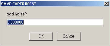
Adding noise provides a very convenient way to generate simulated data, using the experimental data set as a template.
If you have specified for a particular experiment to consider a radial-dependent baseline profile, then you can save this into a file. The filename will be TIN.rxx, and you may want to save it into a special directory for each experiment. The analogous SedfiT function is Data->Save Systematic Noise->Save Noise in File.
As an alternative, you can also access and perhaps more conveniently store the noise parameters using the copy function of SedphaT and pasting the data in a spreadsheet of your favorite plotting program.
![]()
This pops up the submenu:
for organizing model parameters:
1) Save current global parameters in file: This function saves a file to the harddisk that contains the information about the current model. The file will have an extension "*.sedphat_PAR". After saving the model parameters, they can be reloaded, thereby providing a way to restore the exact set of parameters, and a way of storing and documenting the results.
Note that some of the models include local parameters, which are stored in the experiment files (xp - files) [like loading concentrations, meniscus position, etc.]. Therefore, the restoration of the current analysis may not be successful if it is based on saving the model only. For this reason, it is recommended to use the more complete functions for saving configurations.
2) Read global parameters from file: A previously saved set of parameters from a "*.sedphat_PAR" file can be loaded into the current SedphaT session and applied to the data analysis. Note that if the saved model is not the currently selected model, the model can be switched to the one in the file.
Note: from version 4.0: the *.sedphat_PAR files can be applied to currently loaded data by drag-and-drop of this file into the open SedphaT session.
3) Save current global parameters as default: Frequently it is useful to have the parameters of a given model already pre-adjusted according to your interests. For example, if you work frequently with the same set of molecules, it may be very convenient to start up the models already with the correct known molar mass, s-values, etc. This is a convenience, but in the long run saves a lot of time and avoids errors. You can use that also as a quick temporary storage for intermediate results that you want to fall back to in the course of an analysis.
Note: the default files for the different models are all in the directory "c:\sedfit" and have all different names, ending with "*.ini", like "124.ini" for the monomer-dimer-tetramer model. The names are automatically assigned and cannot be changed.
4) Read default global parameters from file: Sometimes the fitting algorithm diverges or the analysis doesn't take a reasonable course. With this function you can quickly go back to your default parameters (or your intermediate results, if you have stored them as default parameters).
5) Set current model as startup default: Beyond customizing the default parameters in each model, you can set the current model to be the default model that SedphaT starts up with.
![]()
Configurations are the subject of this part of the data menu:
For an introduction to the idea of configurations and specific details on the file structure, see Configurations.
1) update current configuration: If the current state of the SedphaT analysis (the model combined with the data) has been saved in a configuration file ("*.sedphat"), this function allows a quick update of this file. This provides a quick way to keep you documentation up-to-date during the course of an analysis. The keyboard shortcut is control-U. If no configuration filename has been saved yet, it will automatically ask for one.
Note that the current configuration name will be lost after a change in either the model or the experiments loaded.
2) save current configuration: Generates a file "*.sedphat" that describes the complete state of the analysis. Information in the sedphat-file are the paths of all the experiment files (xp-files) loaded, the global parameters like vbar(20), and all links between local parameters of the experiments. It will also automatically write a "*.sedphat_PAR" file with the type and global parameters of the current model.
Because sometimes you may want to make different analyses of the same data with different models, and because different models may change the local parameters stored in the xp-file (like meniscus position, etc.) it is advisable to make a new copy of the current xp-files for each configuration. That way, the complete information about the analysis can be stored in a reproducible way, and several alternative analyses of the same data may co-exist.
The name of the current configuration file is shown in the title bar of the SedphaT window.
Note that much of the information stored relies on the exact location of your xp-files and the sedphat_PAR file on your computer. If you move your analysis between different computers, it is best to use exactly the same directory structure. Alternatively, you can edit the sedphat files with the notepad and adjust the pathname of the xp and the sedphat_PAR files.
Do not use directories with white-space characters, e.g. "My Documents", "XLA DATA" or the desktop.
The keyboard shortcut is control-W.
3) read configuration from file: This is a way to restore a previous SedphaT configuration and exactly reproduce an analysis. It reloads the data, the model, the global parameters, and restores all links between the data sets. Be aware that the file structure is important (see above), otherwise SedphaT won't find the data.
The keyboard shortcut is control-C.
You can also associate "*.sedphat" files with sedphat.exe [single right-click on sephat file, select "Open With", "Choose Program", "Browse", find sedphat.exe, and check "Always use the selected program...". This will allow you to simply double click on any sedphat file from within your file manager and start a new copy of SedphaT showing the saved analysis.
4) set current configuration as default startup: This can be useful if you want to continue or extend the current analysis later.
5) reset default configuration: reverses the previous procedure and switches back to the startup default configuration, consisting of no experiments, and the species analysis as the simplest model.
6) copy all data and save as new config: This function allows to make a physical copy of all data belonging to all xp-files loaded in this configuration, and generates a Path-Independent Configuration. This can be very helpful to move data and analysis files to different computers.
Additionally, there are two clipboard operations for configurations: Copy current configuration and paste configuration.
![]()
This closes the program. Results of the data analysis should be stored manually, using either the save fit command, the copy commands, the notebook, or other methods. I would encourage using some partial storage of the local parameters by updating the experiments with the Save All Experiments command (see the Concepts for Getting Started).