
This box appears immediately after loading new data, and can also be accessed at any time from the top-level menu. It contains those local parameters which are more related to the physical configuration of the experiment.
How this box looks depends on the experiment type. Let's start with the
The first line specifies the experiment type. This cannot be changed. (You could edit the xp-file, but I cannot see how this might be useful.)
The second line shows the path and filename of the xp-file and in parenthesis the filenames of some of the experimental raw data.
Line 3 allows to enter any comments, such as a sample ID, buffer composition, or whatever you like to remember about this experiment.
Then follow a number of check-boxes and numbers. Starting from the top left corner:
Active is a check box for making the experiment active or inactive, which controls if this experiment will be included in the global fit and global run functions of the model, or if they will temporarily excluded.
The noise field is the expected standard deviation of the measurement error. Since the global fit will minimize the global chi-square, which is essentially the ratio between the rms deviation of the fit and the measurement error, a low value of the noise entry will make the chi-square of this particular data set larger, and therefore makes its contribution to the global fit more important. Therefore, this is the point where one can determine how to weight the different experiments against each other. The default entry in the noise field will depend on the data type. For more information, follow this link on the measure for the goodness of fit.
Below is a field that contains information on the centerpiece type (2 for double sector, and 6 for six-channel). This information is used for mass balance calculations in sedimentation equilibrium, which are dependent on the cell geometry. Just below is the field for the optical pathlength of the centerpiece. This is usually 12 mm, but short ones with 3 mm are also sometimes used. For DLS data, these two fields can be ignored. The field for rotor type can assume values of 0 (no information), 4 (4-hole rotor), and 8 (8-hole rotor) [this information is used to correct for rotor stretching in the Multi-Speed Equilibrium model. Following is the field no backdiffusion necessary - check this if the data are not influenced by back-diffusion from the bottom of the cell - this will automatically switch off the backdiffusion in Lamm equation solutions of reactive systems.
On the right-hand side at the top are the specifics for the buffer condition: partial-specific volume at experimental conditions (see the Concepts for Getting Started page on v-bars) the buffer density and buffer viscosity (all at experimental conditions). The temperature field by default has the average temperature taken from the scan files, but can be edited and saved.
The default values for the density and viscosity are the standard conditions (water at 20C). Using the input about the experimental conditions, all parameters in SedPHaT will be corrected to standard conditions. This is one of the main differences to SedfiT, which (except for the inhomogeneous solvent models) always reports results under experimental conditions. SedPHaT will always report s-values, D-values, etc. for standard conditions. This is necessary because different experiments may have different experimental conditions. SedPHaT actually calculates with parameters at standard conditions, and for each experiment translates them to the experimental conditions specified in the fields of the Experiment Parameters Box. (If you do not want SedPHaT to make any corrections, accept the defaults (pretend the experiment was already done at standard conditions, in which case no further correction will take place.) But generally it's definitely worth the trouble of looking up the correct parameters - most likely you'll need the anyway sooner or later. Once you've entered them here, save the experiment and you them stored with the data.
New in version 1.9: Once one experiment has been loaded, the default density, v-bar, and viscosity settings will be those of experiment 1.
Moving to the middle row of parameter fields, on the left we find the baseline parameters. The fit baseline checkbox will add a single parameter for a constant offset. For multi-speed sedimentation equilibrium data, this baseline is shared for all rotor speeds. For sedimentation data, it can be useful to check the fit RI Noise box, which adds a 'radial-invariant' offset for each scan in the current experiment. This can take care of the jitter in interference optical sedimentation velocity data, or some baseline shifts between the scans at different rotor speeds in multi-speed sedimentation equilibrium data. The fit TI Noise box switches on a radial-dependent baseline profile common to all scans of sedimentation velocity or multi-speed sedimentation equilibrium data. This can be used to account for systematic spikes in the data, caused by dust or scratches on the windows in absorption optics, or by the common effects of imperfections on any optical surface in interference optical data. The RI noise and the TI noise are calculated by algebraic techniques, for an introduction see the SedfiT tutorial on systematic noise.
In the center are is the section for entering meniscus and bottom of the solution column. They can be optimized in the non-linear regression by checking the box next to the parameters. For DLS data, ignore these parameters (but don't optimize them). You can enter them graphically, too, like in SedPHaT. If you switch on the optimization of meniscus and bottom, you will be asked for upper and lower bounds for these parameters. Please note: set the upper and lower bounds carefully, as the default is not always a good value and may constrain the fit to poor menicus or bottom positions. If you want to change the bounds for meniscus and bottom, uncheck the optimization in the experimental parameter box, close the box, reopen the box, and re-check the fitting marks for meniscus and bottom. This will give you a chance to double-check or modify these values.
Just to the right is the field to redirect men./bot, i.e. to copy the meniscus and bottom parameters from another experiment and use them as parameters of the current experiment. For an introduction to shared local parameters, follow this link. You can switch parameter sharing on for this experiment by checking the box, and entering the experiment number that should serve as a parent experiment (i.e. which provides the parameter values) with regard to this parameter. Sharing will automatically copy any option of the parent experiment to optimize or fix meniscus or bottom. Sharing meniscus and bottom is highly recommended when the data originate from the same solution column.
The bottom fields specify extinction coefficients for a species A (default species in self-association models) and a species B and C (used only for hetero-association models). Note that extinction coefficients will not be used for the non-interacting models. Enter the values in molar extinction coefficients per cm. (Pathlengths will be taken care of automatically by SedPHaT). You can optimize these parameters by checking their box, and you can also share those of another experiment.
Please note: You should not fit both the extinction coefficients and concentration parameters, unless you have essentially fixed one of them through sharing. For an example of multi-wavelength sedimentation equilibrium analysis, see the examples in the introduction to shared parameters.
For interference optical centrifuge data, substitute the molar extinction coefficient with the signal increment. An example: We get ~ 3.3 fringes per mg/ml of solution with a 12 mm pathlength cell. If we have a 100 kDa protein, 1 mg/ml is 10mM. The specific signal increment would be (3.3/1.2)*105/Mol. In general, it would be (3.3Mw/1.2), if Mw is the molar mass of the protein.
The Sedimentation Equilibrium Box
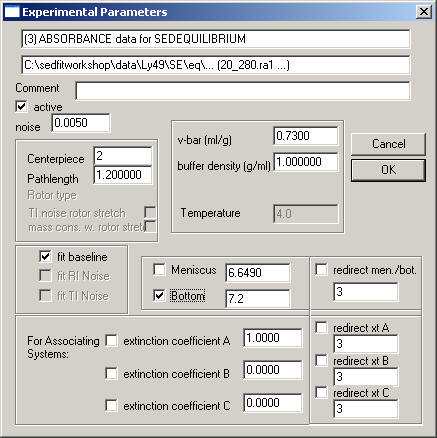
looks like the velocity box, but has fewer entries. RI and TI noise are disabled, since a single equilibrium profile cannot define these noise parameters. Obviously, in equilibrium the viscosity is irrelevant.
The Multi-Speed Equilibrium Box
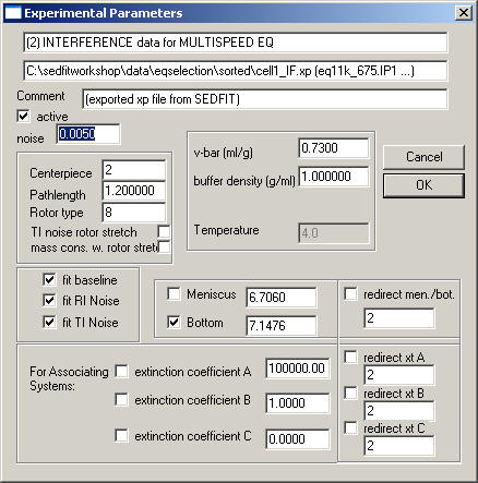
is like the sedimentation equilibrium box, but it can allow RI noise, which in this context is a Baseline that is dependent on the rotor speed, and TI noise, which stands for a radial-dependent baseline. See Analytical Biochemistry 326:234-256 (preprint) for how to use this option. The two fields 'TI noise rotor stretch' and 'mass cons. w. rotor stretch' will determine if the stretching of the rotor is taking into account for calculating the radial-dependent baseline, and for mass conservation, respectively. The extent of rotor stretching will depend on the rotor type, which can assume values of 0 (no rotor information), 4 (4-hole rotor), and 8 (8-hole rotor).
The DLS Data Box

is much simpler. The fields have the same meaning as in the sedimentation models.
The Isotherm Box
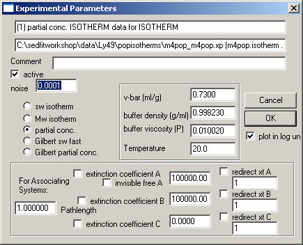
is also similar to the previous ones.
Notice that you have to select the type of isotherm:
sw isotherm: weight-average s-values, determined by integration of c(s) profiles of SedfiT over all species participating in the interaction - this is for all models, independent of the time-scale of the reaction kinetics
Mw isotherm: weight-average molar mass values - can be determined by fitting single-species model of SedfiT to equilibrium data. This is also for all models, independent of the time-scale of the reaction kinetics
partial-conc. isotherm: for slow interacting systems where the c(s) peak positions remain independent of loading composition. Data are amplitudes of c(s), determined by integration of c(s) peaks in SedfiT.
Gilbert sw fast: for fast interacting systems, which can be discerned from c(s) peaks showing peaks positions depending on loading composition. Data are the weight-average s-value of the fast boundary component in c(s), as determined by integration in SedfiT.
Gilbert partial conc: for fast interacting systems, which can be discerned from c(s) peaks showing peaks positions depending on loading composition. Data are the amplitudes of both the undisturbed boundary and the reaction boundary component in c(s), as determined by integration in SedfiT.
For format requirements, see here.
An overview of isotherm analyses in SedphaT can be found here.
The ITC data box

Here, there are a number of specific entries referring to an isothermal titration calorimetry experiment, where one macromolecule is in a cell, to which a binding partner is added in step-wise increments.
cell conc [uM]: This is the initial concentration of interacting macromolecules in the cell.
syringe conc [uM]: This is the concentration of binding partner in the syringe.
recalculate concs: The precision of concentration values in the raw data table exported from the Microcal ITC is not very high. (In part, this is because concentrations are in mM units, as opposed to the micromolar units used here.). The use of the ligand and titrant concentrations from the raw data table can lead to apparent oscillations and noise on the calculated isotherm, due to truncation of concentration values. Therefore, it is generally preferable to recalculate the concentration of ligand and analyte after each titration step, based on the total volume in the cell and the titration volumes in each step.
titration of: Obviously, titration experiments can be performed in different orientations, even for a two-component interaction of A and B. In multi-site models, by convention, the molecule termed "A" is the one having two sites for B. This terminology is part of the model, and cannot be changed. Therefore, the identity of the molecules in cell and syringe must be specified. Clearly, this is crucial for global fits of titrations in multiple orientations. For three-component interactions, one can imagine using a mixture of two molecules in either the syringe or the cell. In this case, the molar ratio of the mixture needs to be specified. For ternary interactions where a reacting binary mixture is in the syringe, the complex formation in the syringe is taken into account.
The "fit baseline" field is straightforward - if checked this adds a floating baseline for this experiment to the parameters. The slope field will determine whether or not a slope will be fitted, in units of kcal/mol per injection.
The button "local incompetent ..." will make the incompetent fraction of A, B, or C, respectively a local parameter for this particular experiment only. This can make sense if several experiments are fitted globally with data that were collected from different preparations or batches of proteins. If the box below the button is checked, the incompetent fraction will be a fitting parameter. The value given in the field is in fractions of total (i.e. enter a value of 0.05 instead of 5%). The max field is a possibility to limit the incompetent fraction. For example, if you know that at most 10% of material is incompetent, enter a value 0.1 here. This constraint for the upper limit of incompetent fraction is active only if the incompetent fraction is determined to be a local parameter.
More information on isothermal titration calorimetry analysis, and format requirements can be found here.
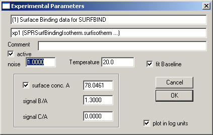
The data-type specific parameters to be entered are:
surface conc. A: This is the signal of immobilized active A. For example, this can be the difference in signal in RU before and after immobilization.
signal B/A and signal C/A: It is possible to account for the fact that the soluble analyte B (or C) have different signal contributions, for example, due to differences in molar mass. In this case, set signal B/A to the ratio Mw(B)/Mw(A).
More information on analyzing surface binding isotherms and format requirements can be found here.
![]()
After the Experiment Parameter Box is closed, for new experiments the fitting limits should be set. This can be made graphically in the SedPHaT window. (Note that a more detailed view is possible using the 'Display->Zoom Into 1 Data Set' function.) I strongly recommend that you save the experiment in an xp-file after all the input has been made. This will allow to conveniently and reproducibly retrieve the entire data selections and settings.
![]()