
As documentation please refer to the following books, which have specific information on SEDFIT and SEDPHAT functions as side-bars nested into the description of theory and experiment of analytical ultracentrifugation (AUC):
New in version 2.0
Sedimentation velocity simulations for reacting systems have been added. This includes self-associating systems, as well as hetero-associating systems both with finite reaction kinetics and with instantaneous equilibrium (on the time-scale of sedimentation).
These models can be used to directly model the sedimentation boundary for reacting systems. It is an alternative to the analysis of the analysis of the isotherm of weight-average s-values and of reaction boundaries of fast reactive systems using Gilbert-Jenkins theory. The boundary modeling extracts more information from the sedimentation data, specifically on the reaction kinetics. However, this comes at the cost of increased susceptibility to all factors that may lead to artifacts in the boundary spreading.
For a detailed discussion of the relative merits of the direct boundary modeling with Lamm equation solutions for reactive systems, Gilbert-Jenkins theory based isotherm analysis, and analysis of weight-average s-values, please see the following references:
J. Dam, C.A. Velikovsky, R.A. Mariuzza, C. Urbanke, P. Schuck (2005) Sedimenetation velocity analysis of heterogeneous protein-protein interactions: Lamm equation modeling and sedimentation coefficient distributions c(s). Biophysical Journal 89:619-634
J. Dam, P. Schuck (2005) Sedimentation velocity analysis of heterogeneous protein-protein interactions: Sedimentation coefficient distributions c(s) and asymptotic boundary profiles from Gilbert-Jenkins theory. Biophysical Journal 89:651-666
A powerpoint presentation on the Gilbert-Jenkins theory and its use for sedimentation velocity analysis of reactive systems can be downloaded from here.
Lamm equation model for reactive systems
The reaction kinetics model simulates the chemical conversion kinetics of the interacting species during the sedimentation process. For systems with off-rate constants > 0.01/sec, the reaction can be considered essentially instantaneous on the time-scale of sedimentation under most conditions (exceptions are theoretically possible for extremely large molecules sedimented at extremely high rotor speed). Therefore the sedimentation profiles become nearly identical to those calculated under conditions where the mass action law is fulfilled instantaneously at all times throughout the cell. This second case limiting is also implemented in Sedphat independently from the reaction kinetics model. [The instantaneous mass action law model for self-associations is a special case of the Lamm equation with locally weight-average s-values and gradient-average D-values, but no such relationship exists for heterogeneous associations.]
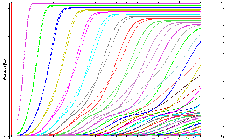
Modeling the boundary shape is the most direct way to extract the entire information content from the sedimentation process. Shown below is an example for the boundaries of a A+B<-->AB reaction with concentrations equimolar at 2xKd, with an off-rate constant of 1x10(-3)/sec (bold lines), in comparison with the same system in instantaneous equilibrium (thin lines), which produces steeper boundaries.
In comparison, the thin lines in the next figure are for an off-rate constant of 1x10(-5)/sec, which produces broader boundaries which already partially separate (the same koff = 1x10(-5)/sec data are plotted again as bold lines).
These differences may be exploited to gain information on the stability of complexes. In the global model, thermodynamic binding parameters can be determined.
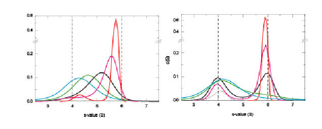
For reactive systems studied by sedimentation velocity, it is a good idea to start with the c(s) analysis of SedfiT , in order to get a feel for the time-scale of the reaction. Generally, experiments are needed over a range of concentrations, covering conditions where species are dissociated and concentrations > 10Kd where they are mostly assembled. If in the c(s) analysis the peak positions remain constant (allowing for the broadening at very low signal-noise ratio) and only the area changes, the reaction is slow on the time-scale of sedimentation. However, if the peak position changes, this indicates a reaction fast on the time-scale of sedimentation. The following normalized c(s) curves illustrate this behavior for a fast (5x10(-3)/sec) self-association reaction on the left, and and a slow one (5x10(-5)/sec) on the right (at concentrations 1/10, 1/3, 1, 3, and 10 times the Kd).
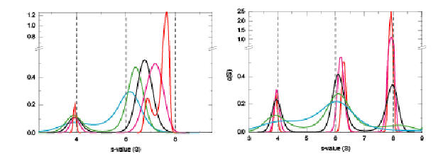
A similar behavior is seen for fast (left) and slow (right) heterogeneous associations (binding constants identical to the previous figure):
The c(s) analysis will aid in estimating the initial values for the s-values, equilibrium constants, and off-rate constants. Further, the integration of c(s) over all reactive species leads to the isotherm of weight-average s-values, which can be analyzed independently to elucidate the reaction scheme, the binding constants, and to estimate the species s-values. This is a rigorous approach independent on the scale of the reaction kinetics. (The relative merits of the direct modeling of the boundary shape versus isotherm analysis has been discussed for rapid self-associating systems in Analytical Biochemistry 320:104-124 (preprint)). For slow systems, where each species population can be identified, integration of all species populations can be an independent approach to analyze the binding isotherm through each species concentrations as a function of loading concentration. For fast reactive systems, SEDPHAT has models for the use of Gilbert-Jenkins theory for the quantitative analysis of the s-value and amplitude of the reaction boundary.
Details of the implementation of the direct boundary model and tips for its practical use in fitting:
Internally, Sedphat will switch automatically between the instantaneous equilibrium and the finite reaction kinetics model if the off-rate constants are equal or faster than 0.1/sec. In other words, if the values for log10(k-) are -1 or larger (e.g., 1), the mass action law based algorithm is used.
In the other extreme, complexes with koff values smaller than -6 (koff < 1x10(-6)/sec) will lead to sedimentation profiles nearly identical to those of independently sedimenting populations of the free and complex species of the loading mixture. (This special case is not internally converted.)
For modeling, it is important to globally model sedimentation data from a range of loading concentrations that lead to the population of all species.
The specifics for the input of the relevant reaction parameters are described in the self-association models and the hetero-association models.
When working with the reactive system models, it may be required to make sure that numeric stability is achieved, and that the simulation is efficient. This can be controlled in the settings of the Lamm equation options. The following points are for optimizing the algorithm and for troubleshooting:
* if the sedimentation velocity data do not include back-diffusion, specify this either in the experimental parameter box, or in the corresponding Lamm equation options field.
* if the simulations are too slow, change the grid size (usually not much below 50 per mm solution column), increase the settings for reaction per step and sedimentation per step (not above 1), and/or set the correction level to the setting 1. This may be required for initial fitting.
* if the simulations do not converge, increase the grid size (e.g., 1000), increase the settings for reaction per step and sedimentation per step (e.g., 0.1), and/or modify the correction level (usually the setting 1 should be best, but 2 or 3 may in some cases be superior).
Currently, hydrodynamic non-ideality not included in the reaction kinetic models. (Exception is the instantaneous equilibrium of self-associating systems.)
All models provide the possibility of adding an additional species that is unrelated to the reactive species. This can be used to describe, for example, a contaminant, or IF signals from sedimenting buffer salts. Concentrations estimates of this un-related species are entered in the local parameters menu. The presence of such components, and their estimated molar mass and s-value may be obtained from c(s) analysis with SEDFIT.