
SedphaT allows to load and analyze data from isothermal titration calorimetry. This can be in the context of a single titration data set, or as a global analysis of several titrations, or as part of a global analysis of different data types.
The preferred method for data import is via NITPIC (http://www.ncbi.nlm.nih.gov/pubmed/22530732, see http://biophysics.swmed.edu/MBR/software.html). This will ensure the highest precision of integration, is completely unbiased, and provides error bar estimates to be used in the SEDPHAT analysis.
In addition, data can be manually imported from software packages that come with the instruments, such as Microcal Origin and the CSC Bindoworks, after pre-processing the raw data of heats versus time into a table of normalized heats per injection. For example, from the Microcal Origin software, find the window that contains a multi-column data table, the first column termed "dh". Export the table of integrated heats per injection into an ASCII file with the extension "*.dat". It will look somewhat like the one shown below. [Make sure the format is tab-delimited like the example below; regional differences in Origin may create comma delimited text files.] From Bindworks, go to the "Area" tab, and use the button to save the table into a file with default extension "bnw".
In either case, the information provided is similar to the following table:
| DH | INJV | Xt | Mt | XMt | NDH | DY | Fit |
| -0.23725 | 2 | 0 | 0.0045 | 0.01562 | -- | -- | -29237.19319 |
| -11.93808 | 8 | 7.01951E-5 | 0.00449 | 0.07832 | -27545.21246 | 1362.23253 | -28907.44499 |
| -12.85444 | 8 | 3.49989E-4 | 0.00447 | 0.14138 | -29836.11227 | -1607.73097 | -28228.38131 |
| -12.12782 | 8 | 6.28203E-4 | 0.00444 | 0.20478 | -28019.54619 | -751.64313 | -27267.90306 |
| -11.23063 | 8 | 9.04839E-4 | 0.00442 | 0.26854 | -25776.5644 | 115.47887 | -25892.04327 |
| -10.10172 | 8 | 0.00118 | 0.00439 | 0.33264 | -22954.28978 | 974.37451 | -23928.66428 |
| -9.42282 | 8 | 0.00145 | 0.00437 | 0.3971 | -21257.05173 | -31.41723 | -21225.6345 |
| -7.81856 | 8 | 0.00173 | 0.00434 | 0.46191 | -17246.39202 | 560.63236 | -17807.02438 |
| -6.7935 | 8 | 0.002 | 0.00432 | 0.52707 | -14683.75699 | -646.07408 | -14037.68291 |
| -5.12402 | 8 | 0.00226 | 0.0043 | 0.59258 | -10510.04268 | 1.06277 | -10511.10545 |
| -3.96208 | 8 | 0.00253 | 0.00427 | 0.65844 | -7605.19219 | 56.99754 | -7662.18973 |
| -3.319 | 8 | 0.0028 | 0.00425 | 0.72465 | -5997.49472 | -422.87428 | -5574.62044 |
| -2.72054 | 8 | 0.00306 | 0.00422 | 0.79121 | -4501.35924 | -387.94407 | -4113.41517 |
| -2.38265 | 8 | 0.00332 | 0.0042 | 0.85812 | -3656.6266 | -556.39922 | -3100.22738 |
| -1.81935 | 8 | 0.00358 | 0.00418 | 0.92539 | -2248.37383 | 141.9495 | -2390.32333 |
| -1.43325 | 8 | 0.00384 | 0.00415 | 0.993 | -1283.13357 | 600.1347 | -1883.26827 |
| -1.282 | 8 | 0.0041 | 0.00413 | 1.06097 | -905.00719 | 608.03931 | -1513.0465 |
| -1.12649 | 8 | 0.00436 | 0.00411 | 1.12929 | -516.21851 | 720.5327 | -1236.75121 |
| -1.02346 | 8 | 0.00461 | 0.00408 | 1.19795 | -258.65884 | 767.61415 | -1026.27299 |
| -0.89437 | 8 | 0.00486 | 0.00406 | 1.26697 | 64.08199 | 926.97654 | -862.89455 |
| -0.91621 | 8 | 0.00512 | 0.00404 | 1.33634 | 9.48372 | 743.39161 | -733.90789 |
| -- | 0.00537 | 0.00402 | -- |
In the above example, we find 21 titration steps, with the following columns:
1) DH, the raw measured enthalpy change for each injection. This column is ignored in SedphaT.
2) INJV, the injected volume in microliters.
3) Xt, the cell concentration of the titrant (the binding partner initially loaded in the syringe) in mM (NOT micromolar) before the injection. This value is used by SEDPHAT in the option "use stored concs" (see below), otherwise the entries are not being used.
4) Mt, the cell concentration of the ligand (the binding partner initially in the cell) in mM before the injection. This value is used by SEDPHAT in the option "use stored concs" (see below), otherwise the entries are not being used.
5) XMt, the molar ratio of titrant to ligand. [This value is read into SedphaT, but will be used for plotting purpose, only.]
6) NDH, the normalized heat per injection. This normaliized heat is used as the data that need to be modeled.
all following columns are ignored.
The last line contains the cell concentration of the titrant and the ligand after the last injection. The last line is indicated by two dashes '--', which has to precede the final value for Xt, as indicated above.
The data in this table for the concentration and the normalized heats are corrected for the effects of dilution of the cell contents due to the addition of the ligand, and the problem that the total volume increases beyond the heat-sensitive volume of the cell.
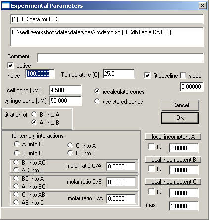
Use the function Data->Load New ITC Data to generate an xp-file for the ITC experiment. Select the appropriate ASCII file generated above. Then, you will arrive at the ITC parameter box
where we have to specify what is titrated in what, as well as the concentrations of all components.
The cell volume if the VP-ITC is 1414.1 microliters, and this is currently assumed as the default for all ITC data. However, it can be changed here. (From the bindworks file, it should automatically adjust to the cell volume information stored in the bnw file.)
Other optional input fields: The "fit baseline" field is straightforward - if checked this adds a floating baseline for this experiment to the parameters. The slope field will determine whether or not a slope will be fitted, in units of kcal/mol per injection. The button "local incompetent ..." will make the incompetent fraction of A, B, or C, respectively a local parameter for this particular experiment only. This can make sense if several experiments are fitted globally with data that were collected from different preparations or batches of proteins. If the box below the button is checked, the incompetent fraction will be a fitting parameter. The value given in the field is in fractions of total (i.e. enter a value of 0.05 instead of 5%). The max field is a possibility to limit the incompetent fraction. For example, if you know that at most 10% of material is incompetent, enter a value 0.1 here. This constraint for the upper limit of incompetent fraction is active only if the incompetent fraction is determined to be a local parameter.
As can be seen above, the concentrations exported by the VP-ITC software are in millimolar, which generates a truncation error in the cell concentrations, which will lead to apparent noise in the calculated isotherms, in particular at high molar ratios. SedphaT provides the option to either use those truncated concentration values and tolerate the noise, or to recalculate the cell concentration values based on the provided cell and syringe concentrations. This will result in a smooth fitted curve, as can be expected. The formula for calculating the concentration of ligand L(i) and titrant T(i) at the start of the i-th titration step with volume dV(i) and the syringe concentration Ts is:
T(1) = 0; L(1) = L0; Vtot(1) = V0;
C(i+1) = C(i)*(1-dV(i)/Vtot(i));
T(i+1) = (T(i)*Vtot + Ts*dV)/(dV+Vtot(i));
Vtot(i+1) = Vtot(i)+dV(i);
For ternary interactions, it is possible to analyze experiments where either the cell or the syringe contains a mixture of molecules. If the syringe contains a mixture of reacting molecules, the heat of pre-existing complexes is taken into account.
The following is an example for the analysis of the above titration. The data can be downloaded from here. Use the function Data->Load New ITC Data, select the downloaded file, enter the loading concentrations of 4.5uM for the cell, and 50 uM for the syringe, let SEDPHAT recalculate the concentrations, fit baseline, and specify that this titration is A into B.
If you peek at the data below, you can see that the inflection point is at a molar ratio of ~ 0.5. This indicates a two-site interaction, which we know is appropriate for the molecules studied.
Note: If we knew that this was a 1:1 interaction, the location of the inflection point obviously would indicate that the loading concentrations are quite a bit off. It is possible to take this into account in SEDPHAT. However, instead of floating an 'n-value', we float the parameters describing the "incompetent fraction of A" and, separately, the "incompetent fraction of B". This requires the model to selected correctly, and we directly obtain the fractional activity separately of A and B. If this was a 1:1 interaction, then we would expect the incompetent fraction of either A or B to be approximately 0.5.
However, let us consider the present titration that of a stable, symmetric dimer into a solution of ligand. Each protomer of the dimer has one site for the ligand, and the sites are identical. In this case we have a two-site interaction of the type A+B+B <--> AB+B <--> ABB (A symbolizing the dimer, B the ligand in the cell). Switch to this model, and look at the parameter box. We can enter an initial guess of the logKa1 to a value 6 (we know it has to be at least in the micromolar range), and the delta-H to about -15 kcal/mol (for high affinity interactions, this is approximately the y-axis intersect divided by the number of sites). We assume that the second site is microscopically identical to the first, which means we leave the value of log(Ka2/Ka1) unchanged at the statistical factor of -0.6 (or 1/4) and keep this fix. Likewise, we set the difference of delta-H from second site and first site to be zero, and we keep it fixed, since there won't be enough information from a single titration to determine any difference in delta-H from the first to the second site. Essentially, we assume that this is a non-cooperative interaction.
(Many models are available in SEDPHAT, to be chosen according to what's known about the system under study.)
The following is the parameter box after the fit has converged:

Next, close this box and invoke the Fit function on the SEDPHAT menu. [The fitting algorithm can be selected in the Fitting Options between Simplex, Marquardt-Levenberg, and simulated annealing.]
This the screen output after the fit has converged:

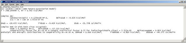
The best-fit estimates for the global parameters are indicated as printed out on the screen. It is a good idea to store this analysis by using the function Data->Save Configuration. This will allow to exactly restore this fit later to the same stage we're at now.
More detailed information can be found in the parameter box:

or by pressing control-T (or menu function Display->Display Themodynamic Information), which will write to the hard disk and display an ASCII file containing the full thermodynamic characterization of the system based on the current best-fit estimates.
As with all other data analysis in SedphaT, the actual values for the fitted line and the residuals are accessible with copy and paste to any spreadsheet.
If you use the function "Save Fit Data", a new ASCII file will be generated in the same format as the *.DAT file exported from Origin.
[It may be of interest to inspect how the fit would look like if we use the 'stored concentrations' from the original DAT-file exported by Origin: We'll find that the global parameters are virtually identical, but the fit looks 'noisy' - this is a result of the stored concentration values having significant round-off error.].
This example illustrated how to use SEDPHAT for a single data file analysis. However, greatly improved parameters can be obtained, and much more complicated models can be fit once we take advantage of the potential of SEDPHAT to perform global modeling to multiple data sets. For example, this can look like the following:
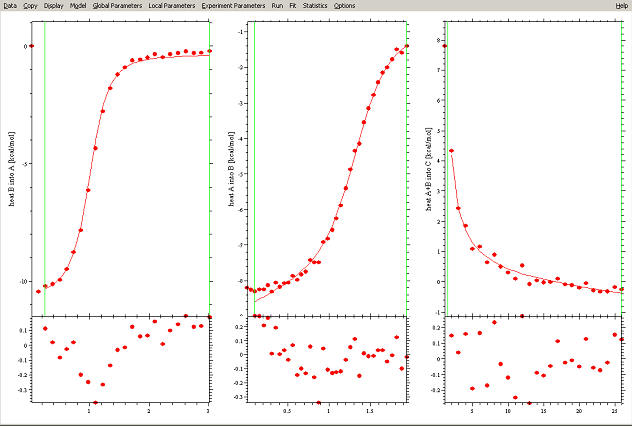
(this is two titrations A into B and B into A, as well as a dilution experiment AB into buffer). Generally, one would want to combine titrations at different concentrations and orientations (for example, binary subsets of ternary systems, as well as ternary titrations like A into mixture BC, etc.)
For more examples, see
J.C.D. Houtman, P.H. Brown, B. Bowden, H. Yamagushi, E. Appella, L.E. Samelson, P. Schuck. (2006) Studying multi-site binary and ternary protein interactions by global analysis of isothermal titration calorimetry data in SEDPHAT: Application to adaptor protein complexes in cell signaling. Protein Science (in press)