back to the tutorial main page
Interpreting and refining the results
First, although the rmsd of 0.0074 seems quite good, the residuals are not evenly distributed. This can be seen from the large residuals in the vicinity of the meniscus, as well as the difference between the data and calculated curves if we zoom in (by pulling a rectangle with the right mouse button) in the meniscus region:
Double-click with the right mouse button (or press ctrl-D) to get back to the previous view.
An even better way to inspect the result is to create a residual bitmap:
Note: this may be checked already by default. If not, invoke the following function:
A little input box will appear for entering the scale of the bitmap, recommending the default of 0.05 for maximal black-white scale:
Hit OK, and you'll see the residuals bitmap in the Sedfit window:
Because the size of the bitmap depends on the radial interval of the data and the number of scans, it may not fit entirely into the Sedfit window on your screen, even if the Sedfit window is maximized on your computer screen. Therefore, to see it in full, one can export the bitmap with the Copy command and paste it into, e.g. PowerPoint. This will show the full bitmap:
Obviously, there is a strong diagonal stripe indicating the mismatch between the data and the calculated curve. At this stage, with large systematic residuals, artifacts can occur in the c(s) distribution.
In order to improve the analysis, we have to refine the calculation.
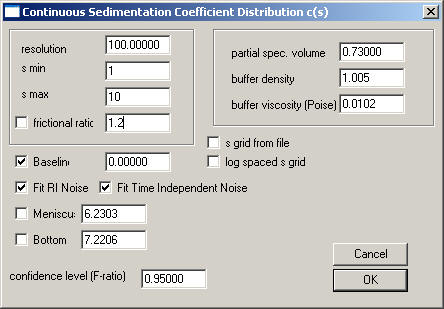
Invoke the Parameter box, and change the frictional ratio parameter to a value of 1.2. The parameter box should look like this:
Execute the Run command:
As can be seen, this makes the main peak sharper (note the scale has changed in the c(s) distribution), and gives a significantly better rmsd. Further, as can be seen from the residuals bitmap, and the systematic deviations in the vicinity of the meniscus are much less.
This demonstrates that the setting of the frictional ratio does not change the gross information (i.e. the main peak at 4-5 S), but it can modify considerably the quality of the fit, and also the details of the distribution for the species of lower abundance.
Therefore, in order to get the true best-fit distribution c(s), we will optimize the settings of the frictional ratio and the meniscus in a non-linear regression.
When working with long-column interference data and a high scan frequency, and with a computer < 1 GHz, I would recommend to reduce the number of scans for the non-linear regression. Do this by loading new files but use only every 2nd or 3rd scan (see Load New Files command):

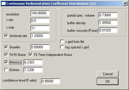
Then go to the parameter box, and enter the following values:
1) Improve the distribution range: The partial peaks at the extreme values of our s-range (i.e. at s-min and s-max) in our preliminary analysis indicate that our s-range was slightly too tight: There was a little bit of a peak visible at 10 S, indicating that there may be something sedimentation with an s-value equal or larger than 10S. Therefore, set the s-max value to 11. Likewise, there is a partial peak visible at 1 S, indicating a possible contribution of a small sedimenting species. Set the s-min value to 0.5.
2) Because we want to use non-linear regression for the frictional ratio, check the box next to this parameter. Do the same thing with the meniscus in order to optimize this parameter. Both of these parameters (which may be slightly correlated) may be responsible for some residual mismatch in the meniscus region.
In the end, the box should look like this:
When pressing OK, a series of input boxes appears prompting you to enter constraints for the variation of the meniscus and bottom. Here, I would recommend to accept the default values.
Next, click on the Fit command in the top-level menu. This will start a non-linear regression using the simplex procedure. The screen output during the fit includes the status of the c(s) analysis in the first 2 lines (or 3 lines, respectively, when using regularization). Additionally, we see in the third line the simplex number (here '3'), and number of steps calculated so far in this simplex (here '0'). The fourth line shows the current rmsd value (this may temporarily increase when restarting a new simplex), followed by the so far best-fit values for the frictional ratio and bottom and meniscus.
New in version 9.2: The graphs for the bitmap, data, residuals, and the distribution can update during the fit (dependent on the preferences settings).
New in version 8.7: it is possible to calculate the ellipsoidal axial ratios corresponding to this best-fit frictional ratio conveniently using the calculator function.
The fit takes approximately a minute or less. Because the simplex procedure can exhibit difficulties in convergence, the fit can be interrupted by pressing the space bar once. This will stop the current c(s) analysis, and will restart the c(s) analysis using the best-fit values.
After convergence, we find something similar to
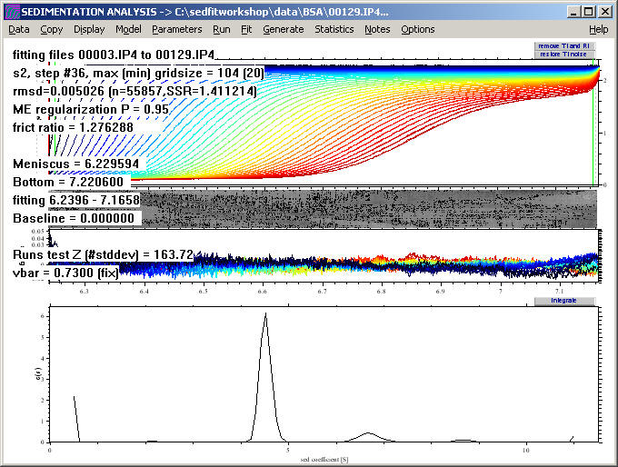
At this point, if the data set had been reduced for the non-linear regression, we could reload the data, using all the files

Please note that the previous best-fit values for the frictional ratio of 1.24 and the meniscus are still maintained.
Click on the Run command (not the Fit command, as we have already performed the non-linear regression) in the top-level menu, and we will get the following output:
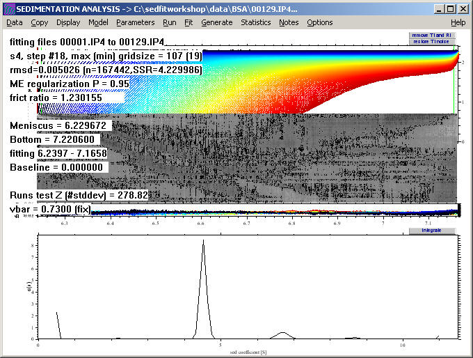
The rmsd of the fit has improved to ~0.005 and the systematics in the residual bitmap is substantially reduced, as visible in the more uniform gray (again, visible best if using the copy bitmap command):

NEW: This distribution can be expanded by using the new command for rescaling the distribution plot in the distribution menu. Also, using the new integration tool, we can calculate the loading concentration and weight-average s-value under each of the peaks.
At this point, we can integrate the distribution. A convenient way to achieve this is via the keyboard shortcut control-M.

This displays little boxes that have the Mw as title and can be clicked. For example, click on the 115 kDa box:
a message appears with further information about the material in this peak

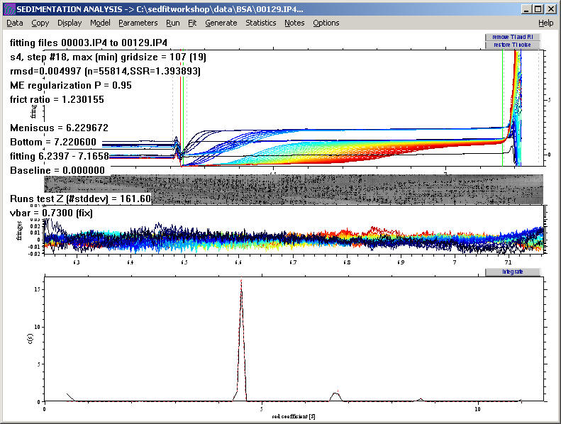
and the sedfit window changes to
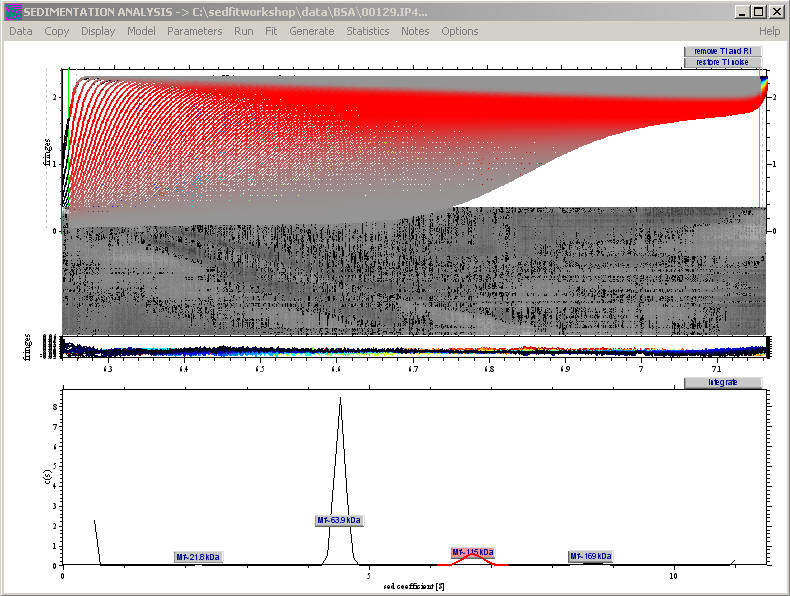
highlighting with the intensity of red where the species from that peak contribute to the raw data. (The intensity of red is governed by the diffusional envelope of the sedimenting species). In the distribution itself, the segment of the distribution is highlighted over which the automatic integration stretches.
Bayesian analysis:
We can use the Bayesian analysis tool to implement the idea that we know all species are pure and monodisperse (i.e. in case we had done a mass spec to ensure the absence of microheterogeneity) and sediment with a single s-value. In this case, control-X automatically places delta-function peaks into the prior probability underlying the regularization.
The result shows sharper peaks, as expected:
Also, a notepad file pops up reminding us how much material is not accounted for in the peaks:
