[ sedfit help home ]
Parameters (keyboard shortcut ctrl-
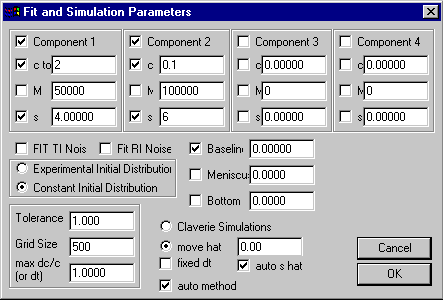
P)This menu item invokes a parameter input dialog box, which will be slightly different dependent on the model used. Each of the parameter boxes are shown in the website of the particular model.
The following information is based on the non-interacting discrete species model, but several elements will be identical for all models.

upper section specifying model-specific parameters,
here c, s and M values of up to 4 components
middle section with experimental conditions
lower section with Lamm equation and
nonlinear regression parameters
The upper sections specifies the parameter specific for the model (see the non-interacting discrete species model for more details on the particular parameter box shown). A convention used in all parameter boxes is that a check-mark next to a parameter field will cause this parameter to be optimized when using the Fit command (for non-linear parameters) or the Run command (for linear parameters).
The middle section contains controls that depend on the experiment, which are common to many models:
1) a checkbox ‘FIT TI Noise’. If checked, the boundary analysis is combined with an unknown radial-dependent background profile that remains constant in time (Time Invariant). This is calculated algebraically and explicit background profiles are used for direct boundary modeling (see systematic noise analysis, and ref 1). Mostly, this function will be used when analyzing interference optical data, although application to absorbance data can occasionally be useful, too (ref 1). It is switched on for interference data by default. After the time-invariant background is calculated, it can be subtracted from the data for better inspection of the fit. Because this TI noise consists of linear parameters, it will be calculated in both the run and the fit command.
2) a check box ‘FIT RI Noise’. If checked, this adds to the model the possibility of a baseline offset that is constant in radial direction, but different for each scan. Like the TI noise, this is calculated algebraically (see systematic noise analysis and ref 3), each time when the run and the fit command are used. It is switched on for interference data by default, because of the small up-and-down displacement (jitter) always involved in sequences of interference scans. Also, the integral fringe displacement sometimes encountered in interference data can count as RI noise. Please note: No correction for jitter or fringe displacement should be performed before the analysis. The best-fit displacements will be result of the analysis, and can be subtracted from the data after the boundary modeling.
3) the field Baseline allows to enter and optimize a constant baseline that is common to all scans and that is constant in radial direction. If this is checked, it will be optimized with each simulation. It is recommended to keep the baseline parameter floated for absorbance data (except when working with very small molecules and small sedimentation rates, when some correlation with the molar mass can be possible if simultaneously floating the bottom parameter).
4) the Meniscus position of the solution column will generally show the radius value that has been graphically determined when loading the files. However, the value can also be entered or changed here. The value of the meniscus position is very important for measuring the sedimentation velocity. When the field is marked, the meniscus is treated as a nonlinear fitting parameter, to be optimized in the fit command. In this case, constraints for a the lowest and highest possible values are necessary (as judged from graphical inspection of the data), and a prompt will automatically ask for these values when closing the parameter box. They should be carefully entered, since the default interval could be off. The range constraints can also be set through the fitting options.
5) the Bottom position of the cell is shown here, as graphically entered. Analogous to the meniscus field, it can be entered or modified here. Also, the bottom value can be treated as a fitting parameter (when checked) to be optimized in the fit command. Also, constraints for a the lowest and highest possible values are necessary when floated, and a prompt will automatically ask for these values (which can be modified through the fitting options). Fitting for the bottom position is very important when back-diffusion of the species from the bottom is modeled, because the exact bottom position is very difficult to locate graphically. Analysis with floating bottom will mostly be required for small molecules with high diffusion constants, at low rotor speeds, or in approach-to-equilibrium analyses. It should be noted, though, that in approach-to-equilibrium analyses at low rotor speed the simultaneous floating of the three parameters bottom, baseline, and molar mass can lead to slight correlation (although generally any two will be well-determined).
6) the radio buttons Experimental Initial Distribution and Constant Initial Distribution. The constant initial distribution is the default, because it corresponds to the conventional loading of the cell. However, the numerical Lamm equation solutions allow for any concentration distribution to be taken as a starting point for the simulation of the evolution. Sometimes, it can be very useful to load an experimental scan as initial distribution, for example when using boundary forming loading techniques, or when convection occurred in the initial parts of the experiment. A detailed description of this approach is given here. It should be noted that with the non-interacting species model, only a single component can be used. (An alternative remedy for initial convection is the use of the differential second moment method.). Please note that when switching to the experimental initial distribution, a warning message may appear, because the corrections for rotor acceleration phase are switched off. This is OK, but it should be remembered that they should be switched on after the analysis session.
The lower section determines the values of parameters that control the solution of the Lamm equation and fitting. Please note: The following control parameters do not have to be changed for the majority of all problems.
In the lower left corner is a series of parameter fields:
1) Tolerance governs the Simplex non-linear regression routine: It determines the (maximum) percent change in the parameter values below which a single Simplex is stopped (see Fit command). The Simplex is then repeatedly restarted, until all final parameter values are within this tolerance in two sequential simplex runs. Default value is 1.
2) Grid Size determines the number of radial increments (dividing the solution column from meniscus to bottom) on which the numerical solution of the Lamm equation is based. Usually, ~ 100 per mm solution column is a reasonable value. Higher accuracy of the Lamm equation solution can be achieved with higher values, but generally the experimental noise is much larger than the error at a discretization of 100/mm. Coarser grids are faster for simulation, but less precise. For complicated situations with time-consuming Lamm simulations, it can be a good strategy to use a coarse grid to get the floating parameter values in a good range, and to use a very high number of grid points only in the end as a final refinement step. This idea is automated if the fitting option of speeding up first Simplex is used; in this case half of the grid size specified here is used for the first round of Simplex optimization only.
3) max dc/c (or dt) has two different functions, dependent on which Lamm simulation algorithm is chosen. In a stationary frame of reference (Claverie simulations), an adaptive time-step driver is used. In this case, the max dc/c parameter refers to the maximum change in any of the concentration values that is desired, and according to which the size of the time-step is adjusted. A larger value of max dc/c effectively increases the time-steps, while a smaller value decreases the time-steps. The detailed algorithm used is slightly more complex, and also depends on the steepness of the simulated boundary.
! If the desired relative change max dc/c leads to too large time-steps, it is automatically reduced.
For the moving frame of reference simulation, this field has no direct function. However, if a fixed dt is chosen, the time-steps in both the Claverie and moving hat algorithm are constrained to the value given in this field (in seconds).
In the middle of the lower section are the controls the choice of the Lamm solution algorithm. Details on these algorithms can be found here.
1) Claverie simulation toggles on the use of the finite element method with stationary equidistant grid as described by Claverie. This works best for small s or low rotor speed (i.e. in cases where diffusion influences are high relative to sedimentation).
2) move hat toggles on the use of a finite element algorithm with a moving frame of reference. This method is preferred for cases of high influence of sedimentation versus diffusion, i.e. for high rotor speed and larger molecules. The input field next to the radio button allows to change the sedimentation coefficient of the frame of reference. However, this input will be effective only if the next check box
3) auto s hat is not marked. The default configuration is auto s hat on, which adjusts automatically the movement of the frame of reference to the sedimentation coefficient of the simulated solute. This will reduce the simulation on the moving frame of reference to diffusion and radial dilution. This algorithm also works automatically with a fixed time-step, which is determined by the movement of the frame of reference. This size of the time-step, however, can be constrained to smaller values (not to larger ones).
4) fixed dt is a checkbox that can be used to constrain the time-step size. The effective value (in sec) will be the one entered in the field ‘max dc/c (or dt)’ (see above).
5) auto method is by default on. This automatically switches during an optimization from the Claverie method at low s to the moving hat method at higher s. The transition point is by default 5 S at 30,000 rpm, with automatic adjustment at higher and lower centrifugal field, but it can be changed using the fitting options.
references
(1) P. Schuck and B. Demeler (1999) Direct sedimentation analysis of interference-optical data in analytical ultracentrifugation. Biophysical Journal 76:2288-2296.