back to sedfit help web    

Size Distribution Analysis

This is only a brief description of the basic concepts.  For more detailed information, see the book https://www.crcpress.com/Sedimentation-Velocity-Analytical-Ultracentrifugation-Discrete-Species/Schuck/p/book/9781498768948

Different levels of sedimentation analysis and the problem of heterogeneity

A general and more formal introduction to size-distributions

An example from the calculation of apparent sedimentation coefficient distributions ls-g*(s)

The principle of regularization

Maximum entropy regularization

Tikhonov-Phillips versus maximum entropy regularization, and the use of Monte-Carlo statistics

The difference between smoothing and regularization

The implementation in Sedfit 

Parameters for size-distribution analysis in Sedfit 

Note: this tutorial does not yet include the information on Bayesian enhancement of the distributions.  For more information, a basic introduction is given in the reference

P.H. Brown, A. Balbo, P. Schuck (2007) Using prior knowledge in the determination of macromolecular size-distributions by analytical ultracentrifugation. Biomacromolecules 8 (2007) 2011-2024

Different levels of sedimentation analysis and the problem of heterogeneity

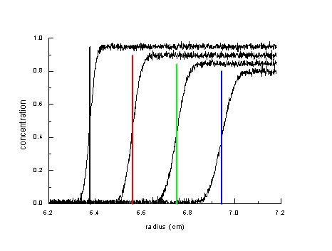
Let's consider the simplest possible analysis of sedimentation data: We look at the displacement of the sedimentation boundary with time.  

The boundary positions at the different times are indicated here by the different color vertical lines.  We could get a very precise s-value if we minimize diffusion effects.  This can be done by applying a high centrifugal field to increase the sedimentation rate so as to form nice and sharp sedimentation boundaries. However, it is clear that this neglects an enormous amount of information contained in the shape of the evolving concentration distributions.  It also does not permit the analysis of molar mass, and the characterization of different protein subpopulations.  

The simplest approach of taking the boundary shape into account is to interpret the spread of the boundary as the result from the diffusion of a single species:  

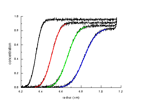
In principle this permits the determination of the diffusion coefficient and the molar mass of the sedimenting species.  However, in practice this approach frequently fails, because it requires the protein under study to be highly homogeneous.  

Unfortunately, in practice we have most of the time heterogeneous mixtures where the root-mean-square displacement from diffusion is in the same order as the separation of species due to their different sedimentation rate.  

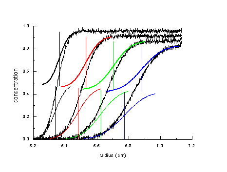
This is illustrated here schematically as the sum of two diffusionally broadened boundaries (series of s-shaped colored lines) with different rates of displacement in the upper and the lower species.  What we experimentally measure in such as situation is the noisy black curve, which is the sum of the components.  Obviously, the boundary spread is broader than the diffusional spread of either component.  In this situation, all known data transformations and extrapolation techniques frequently fail to provide either a good description of diffusion properties of the mixture or a resolution of the sedimentation coefficients of the different species. 

This is the fundamental problem of centrifugal size-distribution analysis:  How can we extract from the experimental boundary shapes reliable information on heterogeneity and diffusion?

A general and more formal introduction to size-distributions

The analysis of distributions addresses the problem that we may not have a homogenous population of molecules in solution, but an a mixture of different molecules.  This can occur, for example, when it is not possible to achieve 100% purification of the molecules of interest.  In this case, analyzing the sedimentation data in terms of a sedimentation coefficient distribution allows to quantify the impurities and focus attention to the main species only.  In other cases, there may be heterogeneity intrinsic to the molecules under study, such as micro-heterogeneity in the glycosylation of a protein, the existence of different oligomeric species of the same macromolecular component, or because the macromolecules are produced by a statistical polymerization process.   

An excellent introduction to the problem of analyzing size-distributions was given by Provencher¹.  The main points can be seen by considering the difference between a direct and indirect measurement.  A good approximation of a direct experiment for measuring the molar mass of a molecule is mass spectrometry (assuming only single charged ions), where we get very precise and very sharp peaks for each species, and size-distributions can (ideally) be observed simply as the envelope of all peaks.  Importantly, the determination of a species of one molar mass does not interfere with the detection of a molecule with another molar mass.  

In contrast, an example for an indirect measurement is sedimentation equilibrium.  Here, what's measured is not directly the molar mass, but instead the radial concentration profile of the molecules, from which the molar mass is calculated by curve-fitting of the type

(1)       

The first line of this equation is the well-known expression for sedimentation equilibrium, and in the second line this is formally simplified into the product of a concentration factor and a characteristic function.  In this particular example, the characteristic function, called a_theo(r,M), describes the shape of the concentration profile of a single species of a certain molar mass M.  If we have a size-distribution instead of a single species, what is measured for a distribution of molecules of different sizes is a superposition of the radial profiles of all species:

(2)         

The resulting analysis problem of deriving the molar mass distribution c(M) from the measured data a(r) is called an inverse problem, and Eq. 2 is called a Fredholm integral equation of the first kind. They are frequently 'ill-posed' if the characteristic function a_theo(r,M) (i.e. the kernel of the integral equation) is smooth and not very much different for different values of M, and if the measurement contains noise:

(3)          

An example of smooth functions are exponentials.  As will be seen below, the difficulty is that in this case, many completely different distributions c(M) can model the measured data essentially equally well.  

Fortunately, in sedimentation velocity the situation is much better.  Here, the characteristic functions are not exponentials, but the Lamm equation solutions, and the analogue of Eq. 3 has the form

(3b)   

(the size-distribution is expressed as a sedimentation coefficient distribution c(s).) Importantly, the measured data are two-dimensional, i.e. they are a function of radius and time, and the Lamm equation distributions L(s,D(s),r,t) predict the evolution in both space and time.  This additional dimension significantly increases the data basis and also the potential for discriminating different species.  However, though not as bad, the underlying problem is still the same.  

Let's go back to the original size-distribution problem c(M) in Eq. 3 to analyze the problem.  If a direct inversion of Eq. 3 was attempted, the particular solution c(M) can contain strong oscillations and be dependent on the details of the noise.  This is very important to understand, as this will also contain the key to solving the problem.  One way of expressing the problem mathematically is that the quantity

(4)         

vanishes if m grows to infinity (for any integrable function K(x,y) -- this is the lemma of Riemann-Lebesgue¹).  What does this mean for our size-distribution problem?  Suppose that a size-distribution c*(M) is a sinus-shaped oscillation c*(M) = sin(2pM/M₀) with a period M₀ . The 'kernel' K(x,y) is in our example the exponential a_theo(r,M).  From eq. 4, it follows that the integral

(5)           

vanishes as the period of the sinusoid oscillation shrinks (M₀ -> 0, corresponding to the oscillations getting higher frequency).  If this integral vanishes, as a consequence, you could add such a high-frequency oscillation to our 'true' size-distribution without changing anything:

(6)       

If we ignore this problem and simply invert Eq. 3, in general we will get such oscillations, to an extent that depends on very small details of the data, i.e. on the noise.  In general, we do not know if some feature of the calculated distribution c(M) is due to these oscillations, or if it is an essential feature of the molecules under study.   

The following will illustrate this point with an example from the apparent sedimentation coefficient distribution, and it will introduce new aspects that will be helpful for solving the problem.

An example from the calculation of apparent sedimentation coefficient distributions ls-g*(s)

One particular simple example for size-distributions is the apparent sedimentation coefficient distribution g*(s)².  The apparent sedimentation coefficient distribution can be defined by an integral equation

(7)            

        with

i.e. as the differential concentration distribution g*(s) of non-diffusing particles, each of which sediments as a step-function U(s,r,t).  (This sedimentation model is described in more detail here.)  How can we calculate the g*(s) distribution in Eq. 7?  We can simply discretize the integral sign in Eq. 7 into a summation

(8)         

which (ignoring the constant scaling factor Ds for the moment) leads directly to a simple linear least-squares problem 

(9)       

that can be directly solved for the distribution g*_i .  Such discretization of the integral equation works for most size-distribution analyses.

How does this work in practice?  The following graph shows four different ls-g*(s) distributions that were obtained from analysis of the data above.  They differ in the discretization (or 'resolution' as termed in the software) of the sedimentation coefficients (how many values between 0.2 and 12.5 S).  

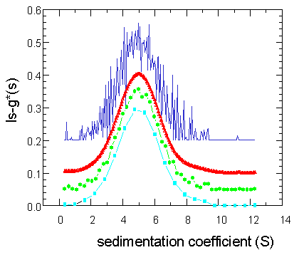
(For clarity of this graph only, the distributions were shown here with different offset.) The cyan colored curve is with a very coarse discretization, using only 20 values.  Because of the coarseness, the quality of the fit (match between the step-functions and the data) is not great, with an rms deviation of 0.034.  The green curve uses 50 s-values, giving a much better fit with an rms deviation of 0.026.  The blue one is calculated with 200 s-values, with a slightly lower rms value of 0.025.  It is obvious that a finer discretization helps only in the beginning, and that further refinement actually leads to significant oscillations.  The better the original integral equation is approximated, the more we see precisely the effect predicted above to produce oscillating distributions.  

At this point, one could simply try to make a compromise between coarseness of the distribution and goodness of fit, and select maybe the green curve as the best one.  However, there's a better way to get a smooth distribution:  The red curve is also calculated with 200 s-values, and it has an rms deviation of 0.0253 -- just slightly higher than the blue curve that was the best-fit solution with 200 s-values (with rms = 0.025).  It is clearly a better representation than either the green or the blue one.  Importantly, the rms deviation of the red curve of 0.0253 is still within the statistical limits of rms values that could be obtained from the 200 s-value analysis (blue curve) just by chance (F-statistics)!  The method used for calculating this red curve is called regularization.    

The principle of regularization

The most important elements of regularization are illustrated in the preceding example:  It is a method to solve integral equations (e.g. size-distributions) without the oscillations, by accepting a slightly worse quality of fit, but still within the statistically acceptable limits.  This can be done by constrained optimization:  instead of minimizing only the sum of squares in Eq. 9, we simultaneously minimize a second property that penalizes the unwanted oscillations.  One important aspect of regularization is that the choice of the penalty term represents our prior knowledge or expectations of a 'good' solution.  As a consequence, dependent on our prior knowledge, there will be different mathematical expressions serving as a penalty term. 

In our example from above, the case of the apparent sedimentation coefficient distribution ls-g*(s), we know that g*(s) is always diffusionally broadened. Therefore, we expect a smooth solution and we can use the higher derivative of the distribution as a measure (Tikhonov-Phillips regularization).  In the following equation, the second term is a discretized approximation of integral over the squared total second derivative of the distribution:

(10)       

The factor a helps to balance the two goals of achieving a good fit and getting a small total second derivative.  This balancing process can be done in the following way:  First, we calculate the unconstrained solution (setting a = 0); this will give the overall best fit, but will contain oscillations (in our example above the blue curve, rms = 0.025).  Then, using statistical principles of how much the rms error can fluctuate for a given number of noisy data points just by chance (see F-statistics), we calculate what increase in the rms error would correspond to a probability that just matches a preset confidence level (in our case 0.0253 on a 68% confidence level).  Now we slowly turn on the constraint.  What happens is that the rms of the fit increases for values a > 0 (because the unconstrained solution was by definition the best-fit). By carefully adjusting a, we can match the rms increase that we would statistically tolerate on a given confidence level. [This rms increase is typically in the order of < 1%, dependent on the number of data points, this can be calculated separately using the calculator.]  

This procedure can be illustrated if we imagine the space of all possible distributions, arranged according to the rms deviations by which they describe our data under consideration.  The overall best-fit distribution has likely positive and negative values, but we only want to consider the subset of distributions that are entirely positive (squared area).  Of those, the blue one has the best rms.  A further subset of the positive functions are the ones that are smooth and positive.  Increasing smoothness leads to higher rms, therefore smoother functions are further away from the overall best-fit.  We make a circle around all functions that have a statistically acceptable rms value. The function that we calculate by regularization is the one just on the edge of this circle, within the subset of smooth and positive functions. 

Maximum entropy regularization

As mentioned above, different regularization procedures emphasize different expected properties of the distribution.  If we do not expect the distribution for principal reasons to be smooth (like the ls-g*(s) distributions), other regularization terms can work better.  One regularization that does not assume smoothness, but uses parsimony in a different sense is maximum entropy.  Here, we maximize the entropy of the distribution calculated as the integral over c lnc, which is the Shannon entropy of the distribution.  In the context of distribution of Lamm solutions c(s), this will take the following form:

(11)         

(where c(s) is the sedimentation coefficient distribution, and L(s,D(s),r,t) are Lamm equation solutions for each species with sedimentation coefficient s and an estimate of the diffusion coefficient D(s), and a is here again the regularization parameter with the same properties as above.)

What is the motivation for choosing this regularization functional?  Because the integral over the expression c lnc is a measure of the information content (4,5), what this regularization favors is the distribution with the minimal information.  A Bayesian approach is used (i.e. a statistical formalism which allows the use of prior probabilities in the data interpretation), with the prior assumption that in the absence of other information, all s-values are equally likely.  (Some modifications in this prior assumption can be build in.)  The connection to the term 'entropy' is that the sum over c lnc corresponds to the number of 'microstates' that can generate a distribution.  We choose the distribution that has the minimal information (maximal entropy) of all distributions that fit the data equally well within our pre-defined confidence level.  This will produce the distribution with the minimal information necessary to explain the data.  According to the principle of Occams razor, this will reduce the likelihood of over-interpretation of the data.  

Maximum entropy regularization is very widely used in many different physical techniques, because it has many useful properties.  One important property is that maximum entropy tolerates isolated sharp peaks, thus making this the regularization of choice for size-distribution analysis of mixtures of discrete particles.  Another useful property is that the entropy is a global property of the distribution, and it does not make use of neighborhood relationship of different s-values (in contrast to the second derivative regularization shown above).

Tikhonov-Phillips versus maximum entropy regularization, and the use of Monte-Carlo statistics

Both Tikhonov-Phillips and maximum entropy regularization select the most parsimonious distribution from the set of all that give statistically acceptable fits of the data (within the predetermined confidence interval).  In principle, therefore, both are valid results of the analysis.  

They differ, however, in the choice of the best distribution among all possible ones, on the basis of different prior knowledge about the distribution.  Parsimony is defined as small total curvature in the second derivative Tikhonov-Phillips approach, whereas it is taken as the least information content in the maximum entropy method.  There are situations where we know that either one method would fit better to the sample under study. 

Situations where we expect to obtain smooth distributions are better described by the minimal second derivative.  These are, for example, the apparent sedimentation coefficient distribution ls-g*(s) (which for fundamental reasons is diffusionally broadened and therefore cannot have sharp peaks), and the study of broad distributions of synthetic polymers (where we may know that the statistical nature of the synthesis leads to a quasi-continuous size-distribution without sharp peaks).  A possible disadvantage of the second derivative regularization is that sharp peaks will be broadened.

On the other hand, maximum entropy does allow for a limited number of very sharp peaks, and is therefore a very powerful model and the method of choice for a mixture of discrete macromolecules.  Known limitations of maximum entropy are a tendency to merge two very close peaks, and a tendency to produce oscillations if applied to broad distributions. 

Because both methods result in statistically acceptable fits, it is also legitimate to chose empirically which method works best for a given problem. However, I recommend to clearly state (e.g. in Materials and Methods) which regularization method was chosen, and also what the predefined confidence limit was.

One way to explore the space of statistically acceptable fits is the use of Monte-Carlo statistics. In this method, many data sets are generated that are very similar to the experimental data but differ in the details of the noise.  A statistical analysis of the set of distributions obtained helps to quantify the effect of noise on the best-fit distribution.

The difference between smoothing and regularization

When considering the second-derivative regularization described above, one could be tempted to mistake regularization for a smoothing operation.  Despite the fact that maximum entropy can allow sharp spikes in the size-distribution, which clearly contradicts this notion, it is worthwhile to clarify the fundamental differences between smoothing and regularization.  

Most importantly, smoothing introduces bias into the result because it makes uncontrolled changes.  There is no feedback step that allows to assess if the smoothed distribution really represents the original data.  Such a feedback step is included in the regularization, making it statistically sound.  A confidence level is predefined, and the parsimony of the solution is adjusted only within that predefined limit.  This makes regularization a rational method for identifying the essential features of the distribution, rather than a method that makes the result look 'better'.  

The implementation of size-distribution analysis in Sedfit

In the following, we describe in detail the calculation of the distribution of Lamm equation solutions c(s).  In this approach, we model the data as a superposition of solutions to the Lamm equation L(s,D(s),r,t):

(12)             

All distributions models in Sedfit are implemented with the same basic strategy, although they may differ in the kernel (i.e. the single-species model function) in different models.  The first step in the calculation is the discretization of the integral into a summation, as 

(13)       

where we have discretized the s-values in a grid of N values (resolution, usually between 50 and 300) between a minimum value (s-min) and a maximum value (s-max).  Automatically, this discretization causes the distribution function c(s_k) to be represented by N values c_k. Also indicated as discrete values are here the experimental data points a at the radii r_i and the time of the scans t_j.  We can consider systematic noise by including terms for time-invariant noise b_i for each radial value and radial-invariant noise for each scan b_j.  

First, the model functions L(s_k,D(s_k),r,t) are calculated for each grid point s_k and stored in the memory.  This may require substantial amounts of RAM, which is why at least 128 MB are recommended for these analyses.  Obviously, this step takes longer for larger values of N. 

Equation 13 is linear, and as described in the section on systematic noise for the direct boundary modeling with discrete species (Eq. 6), we obtain a linear equation system for the unknown concentrations c_k.  We can formulate this equation system as a symmetric normal equation

(14)       

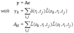
with the inhomogeneity y, the normal matrix A, and the concentration vector c.  The hats over the quantities a and L denote here the transformations for the systematic noise analysis (combine Eq. 3 and 8 in systematic noise page).  Calculation of the normal system (A and y) is the second step of the calculation.  Each element requires summation over all data points, which can be quite computationally extensive, for example, with interference optical data which can easily have 100,000 data points.  Because this is a N x N system, this effort increases quadratically with N. 

This is followed by solving the quadratic linear system.  Sedfit uses the Cholesky decomposition.  There is an easy way to ensure non-negativity of all concentration values algebraically with the algorithm NNLS from Lawson and Hanson (ref 6), adapted for use with normal equations.  This step is very fast and stable even for very large N.  This unconstrained solution allows to evaluate the chi-square of the fit.  Using the predefined confidence level and F-statistics, we can also calculate the chi-square increase that we want to achieve by regularization.

With the abbreviations from Eq. 14, the constrained size-distribution problem for Tikhonov-Phillips regularization by second derivative is  

(15a)       

where B denotes the square of the second derivative matrix (as given in 18.5.12 in ref 4).  Because this is still a linear equation system, it can be solved easily for any value of the regularization parameter a, and the resulting chi-square of the regularized solution is calculated.  A root-finding algorithm is used to adjust a to yield exactly the predefined chi-square.

The maximum entropy regularization is more complicated.  This problem is nonlinear, and with the abbreviations of Eq. 14, can be written as

(15b)       

Sedfit uses a Marquardt-Levenberg algorithm to calculate the minimum of Eq. 15b for any value of a.  Because we already have the concentrations c for the unregularized solution, we take this as an initial starting guess, and chose first a very low value of a.  This will lead to a very small increase in chi-square.  Sedfit increases a in small increments, each time using the concentrations from the previous a-value as a new starting guess.  The chi-square increase is monitored, and the procedure is stopped when the preset value is reached.  Although there may be several hundred unknown c-values involved in this nonlinear problem, the method describes starts from very good starting guesses, and proceeds in many steps with only small changes of a in each of which only very small adjustments in the concentration values need to be made.  Essentially, we move the concentration values 'adiabatic' from the unregularized to the regularized solution, making use of the continuity of the best-fit concentration as a function of a.  

For the maximum entropy method, this root-finding during the regularization is the third major computational task, and Sedfit makes screen outputs that allow to monitor progress (the value of a, the entropy, and the P-value corresponding to the current chi-square increase). 

After the concentration values c(s_k) are calculated, their sum corresponds to the total loading concentration.  This is because during the discretization of Eq. 12 in the form of Eq. 13 ignores the constant factor Ds (that would originate from the differential ds of the integral).  In order to really get the solution of the original integral equation, the distribution is finally rescaled, such that the integral will correspond to the loading concentration.  This can introduce changes of the distribution shape, if the underlying grid points s_k were not chosen equidistant (as is the case, e.g. in the molar mass distribution models, where the M-grid is spaced with a 2/3-power). 

Parameters for size-distribution analysis in Sedfit

Several parameters in Sedfit are common to all size-distribution models.  These are related to the range and discretization of the distribution, and to the regularization.

resolution: This is the number of values between the minimum and maximum of the distribution range.  This number N controls the resolution of the distribution.  For example, for sedimentation coefficient distribution with s-min = 3 S and s-max = 13 S, a resolution value of N = 100 would mean that the s-grid has increments of 0.1S.  Obviously, a larger number is required for covering a larger range, while a small value may be sufficient for a small range.  The computation time increases quadratically with N.  Values can theoretically range from as little as 10 to 1000, although practical ranges are 50 - 300.

s-min:  (corresponding to M-min, D-min, or R-min for molar mass, diffusion coefficient, or Stokes-radius distributions)  This is the smallest value of the distribution.  The value should be well below the smallest s-value that occurs in the sample.  For very small s-values (< 1S), dependent on the rotor speed, a correlation with the baseline parameters can occur, but this is not a problem for the interpretation of the rest of the distribution.

s-max: This is the largest value of the distribution.  It should be larger than the largest species in the distribution.  If the calculated distribution shows a increase toward s-max, most likely there are larger species present, and the value of s-max should be increased. 

confidence level (F-ratio): This parameter controls the amount of regularization used.  It has a different meaning for different ranges:  From 0 to 0.5, no regularization is used.  Values from 0.5 to 0.999 correspond to probabilities P (confidence levels).  From these P-values, the desired chi-square increase allowed for the parsimony constraint of the regularization is calculated with F-statistics.  A value of 0.51 will cause very little regularization; values of 0.68 to 0.90 would correspond to commonly used confidence levels (usually, with 50 scans or more the chi-square increase corresponding to a probability of 0.7 is of the order of 0.1%), while values close to 0.99 would cause very high regularization.  The relationship of these values with probabilities can be examined using the F-statistics calculator.  If numbers > 1 are entered, they are taken directly as chi-square ratios (as there are no probabilities > 1).  For example, a value of 1.1 will result in regularization with 10% chi-square increase.  (In this way, chi-square increase values can be used without utilizing the F-statistics.) 

Another control common to most size-distribution models is the choice of regularization procedure, i.e. between Tikhonov-Phillips 2nd derivative and maximum entropy regularization.  Some guidelines for this choice are given above, and the setting can be changed using the size-distribution option menu.   

Finally, most of the distributions require additional parameters that are characteristic to the model.  For example, because the Lamm equation solutions require two parameters, s and D, the diffusion coefficients must be estimated for each s-value.  This estimate can be made in different ways, which reflect different prior knowledge or prior assumptions on the sample, or approximations.  These are explained in the help-pages of the c(s) distribution model, c(s) with prior knowledge, c(M) distribution model, and c(M) with prior knowledge.  

More practical information can be found in the tutorial for size-distribution analysis.

It should be noted that corrections for compressible solvents can be applied without further difficulty. 

References:

1. S.W. Provencher. (1982) A constrained regularization method for inverting data represented by linear algebraic or integral equations. Comp. Phys. Comm. 27:213-227

2. P. Schuck and P. Rossmanith (2000) Determination of the sedimentation coefficient distribution g*(s) by least-squares boundary modeling. Biopolymers 54:328-341.  

3. P. Schuck (2000) Size distribution analysis of macromolecules by sedimentation velocity ultracentrifugation and Lamm equation modeling. Biophysical Journal 78:1606-1619. 

4. W.H. Press, S.A. Teukolsky, W.T. Vetterling, and B.P. Flannery. (1992) Numerical Recipes in C. University Press, Cambridge

5. A.K. Livesey, J. Skilling. (1985) Maximum Entropy Theory.  Acta Cryst. A41, 113-122

6. C.L. Lawson and R.J. Hanson. (1974) Solving Least Squares Problems. Prentice-Hall, Englewood Cliffs, New Jersey

web pages related to this topic:

tutorial for size-distribution analysis, 

example for using Sedfit

ls-g*(s) distribution

c(s) distribution model, and c(s) with prior knowledge

c(M) distribution model, and c(M) with prior knowledge

ls-g*(s) distribution model, extrapolation of ls-g*(s) to infinite time, van Holde-Weischet analysis

compressibility of water and organic solvents