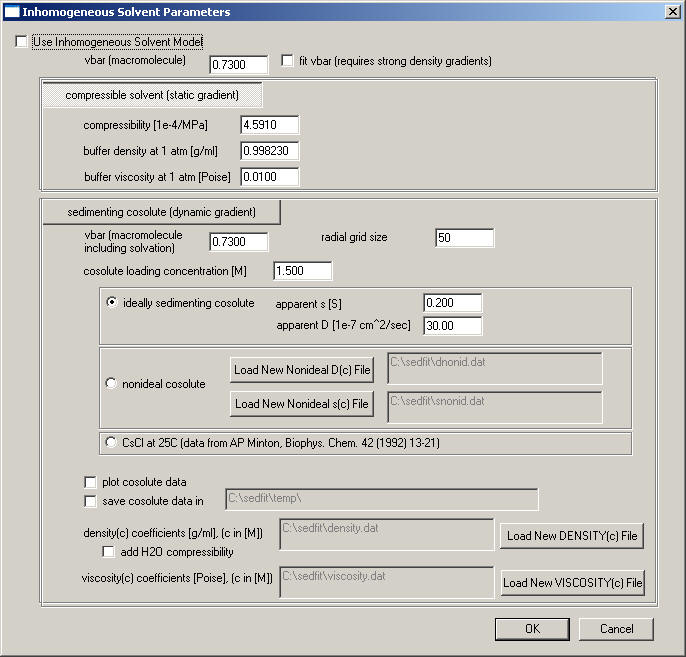
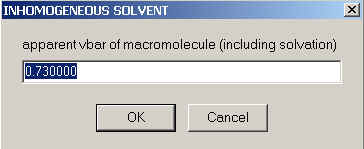
Note, starting from version 11.6, the input has been simplified into a parameter box
. The required values are the same as explained below.
Several different variations of inhomogeneous solvents have been incorporated in Sedfit for simulation and fitting. They are:
* compressible solvents (water and organic solvents)
* dynamic density gradients (generating by high concentrations of sedimenting co-solutes)
* linear gradients (e.g. pre-formed gradients in preparative ultracentrifuges)
* constant solvent (for solvent corrections only, testing)
Using these models requires switching Sedfit into a different mode. Please read the following instructions carefully.
1) For references on the theoretical background with examples of the use of the inhomogeneous solvent models, please see the following two publications:
P. Schuck (2003) A model for sedimentation in inhomogeneous media. I. Dynamic density gradients from sedimenting co-solutes. Biophysical Chemistry 108:187-200
P. Schuck (2003) A model for sedimentation in inhomogeneous media. II. Compressibility of aqueous and organic solvents. Biophysical Chemistry 108:201-214
For the compressibility of water and organic solvents, please see also the tutorial page.
Although
the theory and practice will be developed somewhat below, I recommend to consult
these references, because the following is more concerned with the organization
and use of these models
2) Note: All these models will make the corrections of density and viscosity to refer to water, 20C. This deviates from the convention used throughout the rest of Sedfit.
This breach of the standard convention is required due to the nature of these simulations: In essence, the Lamm equation is solved considering a radial-dependent density and viscosity
![]()
(ref) that transform the underlying D20,w and s20,w values of the macromolecular diffusion and sedimentation coefficients from the standard conditions locally to experimental values. The local density and viscosity corrections are expressed here through the factors a(r,t) and b(r,t). These can vary throughout the solution column, in a way that depends on the specific solvent mode. The radial-dependence of a(r,t) and b(r,t) is incorporated into the finite-element solution of the Lamm equation (ref). [For the case where there are density corrections only from compressible solvents, analytical solutions of the Lamm equation for non-diffusing species are available (ref).]
3) The inhomogeneous solvent mode in Sedfit is either switched on or off. You can see the current status by watching the checkmark on the menu:
and from the first line of text output after fitting, e.g.
4) SWITCHING ON: The inhomogeneous solvent models are selected in a sequence of yes/no questions. (Sorry, that's poor programming style, I know, but it works for now...)
That means that if you make a mistake in the selection, you have to go through with it, then switch the inhomogeneous solvent model off (see below), and then start over again with selecting the correct inhomogeneous solvent mode.
This is how it looks like:
this will bring to the compressible solvent mode:

to the dynamic density gradient from a sedimenting co-solute:
to a linear pre-formed stable gradient:
to a constant solvent (but with buffer corrections)
Selecting any of them will terminate this sequence and lead to a series of questions regarding the specifics of the particular model (see below or follow the bookmark links).
Even if you don't choose any of them, you have switched ON the inhomogeneous solvent mode. You will get a warning that the macromolecule are considered incompressible,
You will need to supply the (apparent) partial-specific volume of the macromolecule
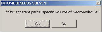
and will be asked if you want to fit for it (i.e. treat the apparent v-bar as a floating parameter to be determined by non-linear regression).
Please note that this only makes sense if there's an appreciable density gradient across the cell. (Otherwise, this will result in non-sense due to correlation with the molar mass parameters - Sedfit will not be able to assist you in this judgment other than providing statistical tools for error estimation.)
Finally, you will get a warning that you have switched Sedfit to the inhomogeneous solvent mode, in which all s and D values are corrected to water, 20C values. For convenience, the parameters of the non-interacting model are transformed to w,20 values automatically:
Please note that when using c(s) or c(M) in the compressible solvent mode, the entries for v-bar, density and viscosity in the parameter box refer to normal conditions (water, 20C) and should not be changed.
5) SWITCHING OFF: To switch back to the normal mode for homogeneous solvents without any solvent corrections, select the menu again.
The menu for Inhomogeneous Solvents is simply a toggle. You switch off this mode by selecting it again when it shows the checkmark:
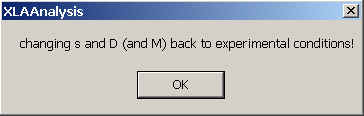
A message will appear that all s and D-values are now back in experimental conditions. For convenience, the parameters in the non-interacting sedimentation model are automatically transformed back to the experimental conditions.
Note that after that, the checkmark disappears, indicating the normal Sedfit mode.
6) The specific operation and required parameters depends on the particular model:
The compressibility of water can cause errors in the s-values and M-values from sedimentation velocity of proteins up to a few percent. Larger errors are encountered when using organic solvents or proteins with higher than usual v-bar. An overview of this problem and how to correct for it can be found in the tutorial, and in this reference.
After selecting this solvent mode, a warning will appear:
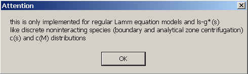
This solvent mode is implemented only for use with the non-interacting species model, the ls-g*(s) distribution, and the c(s) and c(M) distributions. Use with any other models, such as self-association models will produce undefined results. (There's no fundamental problem with those models; it just hasn't been implemented yet.) When dealing with self-associating species, however, what can be done is the strategy of determining weight-average sedimentation coefficients from integrating c(s) or ls-g*(s) (see ref).
First, we need to characterize the solvent. You need to enter it's density under normal pressure, which will be assigned the density at the meniscus.
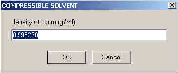
The default value shown here is the density of water at 20C. Please note that density and pressure distribution throughout the solution column are calculated as
(ref) (with r0 the density at 1 atm, k the compressibility, w the rotor speed, r the radius and m the meniscus position). One question is - how should we deal with co-solutes that increase the density throughout but where we don't have data on how they affect the compressibility? From the equations above we can see that r0 is a multiplicative factor for the compressibility. I suggest entering for r0 the true density of the solution at 1 atm (e.g. a value of ~1.005 g/ml for PBS), and then to diminish the compressibility value proportionally. Of course, the latter adjustment of the compressibility value makes sense only if you know the compressibility with a precision better than 1%, and in terms of the overall effect we're talking about a < 1% correction of a few percent... probably not worth the bother. Therefore, I would probably enter here the density of the solution including salt contributions etc.
The solvent compressibility is asked next:
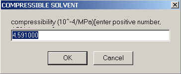
When reading these values from published tables it's important to note that it has weird units, and asked here is the value in 10-4/MPa. In these units, the numeric value for water is 4.591 (the default, as shown), and it is 8.96 for toluene, and can reach up to 15 or so for the more compressible organic solvents. Note that the difference between organic solvents and water is not very much - only a factor of 2 - 3 !
It follows the viscosity of the solvent, in units of Poise
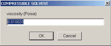
The default here is again the value for water. There are no corrections made in Sedfit for pressure-dependence of the viscosity. That's not for any particular fundamental reason, but just for a lack of data. (However, for non-diffusing species there is a nice analytical solution of the Lamm equation if the viscosity changes can be neglected.) Future improvements may include pressure-dependent viscosity terms.
The second set of questions are regarding the macromolecule. It is assumed to be incompressible. For proteins, this is a good first approximation, as their compressibility is generally less than 10% the compressibility of water.
Then, the (apparent) partial-specific volume of the macromolecule is entered
and it will be specified if that is known or should be treated as an unknown parameter to be optimized in the fit:
You need to be careful in the compressible solvent mode with fitting for v-bar: Although for proteins with common partial-specific volume values sedimenting in aqueous solutions, the density gradient can produce significant deviations from the ideal boundaries expected for incompressible solvents, the effects are very likely far too small to overcome parameter correlation and permit a reliable determination of the protein partial-specific volume. However, much larger effects are observed with protein complexes that have densities closer to water, or with other macromolecules in more compressible solvents; this has not been explored yet.
Dynamic self-forming density gradients are somewhat more complicated to deal with. Sedfit calculates the sedimentation (non-ideal if necessary) of the co-solute, and keeps track of the evolution of the local density and viscosity caused by a given local co-solute concentration. It synchronizes the sedimentation of the macrosolute(s) with that of the co-solute, applying at each time the locally required density and viscosity corrections.

This message reminds that this sedimentation mode is only implemented for non-interacting Lamm equation models, including c(s) and c(M). (No simple solution exists for non-diffusing species, which was possible for the compressibility corrections.) The possible models also include analytical zone centrifugation configurations.
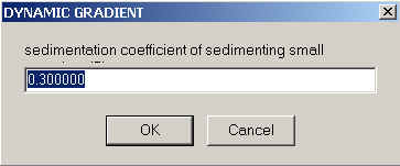
The first set of questions is to characterize the co-solute. It can sediment ideally or non-ideally:

For ideal sedimentation, what you need to enter then is the sedimentation and the diffusion coefficient of the co-solute under experimental conditions.

Where do we get these values from? Simply by running a separate experiment in the same run with the co-solute only, preferably scanning with the interference optics. Modeling of the observed fringe displacement profiles with a single non-interacting species model, using the option to fit s and D. If you use the same co-solute concentration as in the sample and can get a reasonably good fit with the single-species model, then these s- and D-values are sufficient to describe the redistribution of the co-solute.
NOTE: One caveat here is that s-values and D-values of very small molecules can be correlated with the loading concentration parameter (even stronger correlation will be observed for continuous distribution models, which are not really useful or appropriate in this case). The best strategy to avoid this correlation is to run a synthetic boundary experiment.
If you cannot fit the data well with a single-species model, or if you have sufficient data on the concentration-dependence of s and D of the co-solute, you should use the non-ideal sedimentation model. In theory, for non-ideal sedimentation, the concentration-dependence of the diffusion and sedimentation coefficients of the co-solute can be described with activity coefficients
![]()
and
![]()
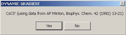
(ref). In practice, however, it's straightforward to just use a polynomial interpolation of experimentally measured D(c) and s(c) data. For convenience, the experimental data for CsCl compiled and interpolated in Biophys. Chem. 42 (1992) 13-21 have been implemented.
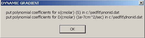
If you're not working with CsCl as a densifying co-solute, you can specify the concentration-dependence of s and D by putting the polynomial coefficients in two files in the directory c:\sedfit, one called snonid.dat, the other dnonid.dat.
The format is the following: Consider the dependence of s and D in molar units as a power series
The files should be in ASCII format with 1 column, with the parameters s1 the first, s2 the second, s3 the third row, etc. (and analogous for D). There can be as many parameters as you need to describe the concentration dependence sufficiently well for the relevant concentration range.
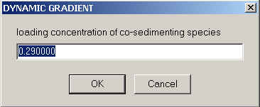
In any case, if non-ideal or ideal sedimentation of the co-solute, we need to enter the loading concentration of the co-solute in MOLAR UNITS (note this is NOT in signal units).
Having specified the sedimentation properties of the co-solute, we need to say how the solvent density and viscosity is going to change as a function of co-solute concentration. This is done also by writing ASCII files to the directory c:\sedfit.
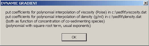
The files are also numbers in a single column, with up to 5 rows for the relative viscosity in viscosity.dat, and up to 6 rows for density in density.dat. Each corresponds to the coefficients a1, a2, a3, a4, a5 (and a6) in the formulas
as used in John Philo's SEDNTERP. The concentration units are MOLAR UNITS, the relative viscosity is dimensionless (you can take the viscosity in Poise and divide by 0.01002 Poise), the density is in g/ml. Make sure the exponents do not already incorporate the power of ten factor in the preceding formula - SEDFIT will multiply the the coefficients with the given powers of ten and the powers of the molar concentration to arrive at the local density and viscosity. Examples are the files density.dat and viscosity.dat. If there is other co-solutes in addition to the high-concentration densifying one, I would suggest the approximation to consider the viscosity and density increments additive. In this case, you can correct the coefficients a1 to account for the additional co-solute (increase the tabulated value of the high-concentration co-solute by the density increment of all the other co-solutes).
Note: the density and viscosity values at concentration 0 should be those under experimental conditions without co-solute, i.e., account for all other (non-sedimenting) co-solutes and temperature effects.
In order to better understand the simulation, it is possible to plot the molar concentration distributions of the sedimenting co-solute
An example of this for 1.5 M CsCl at 50,000 rpm is shown here:
(note the co-solute distribution shown in blue, is plotted only during the simulation)
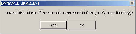
For a more permanent record of what the co-solute did during the sedimentation, you can save the molar concentration distributions in files (synchronized in time with the data files to be modeled) in the directory c:\temp.
Finally, to make the sedimentation more precise, we can take into account the compressibility of water. This can be significant, for example when evaluating buoyant density gradients.
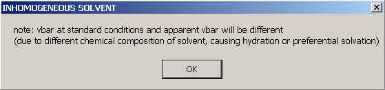
The remaining parameters are for the characterization of the macromolecule. In the presence of a high concentration of co-solute, we have to consider that the macromolecule may be solvated in a way that adds additional buoyancy or mass to the effective sedimenting particle (the latter understood as the solvated macromolecule). This is certainly the case for proteins in high salt, sucrose, glycerol, etc. To account for this, we distinguish the 'apparent partial-specific volume' of the sedimenting solvated particle (which is such that 1-vbar(app)*rho = density increment drho/dc) from the partial-specific volume of the macromolecule under standard conditions (water, 20C):
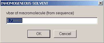
First, we specify the partial-specific volume under standard conditions:
Next, we enter the apparent partial-specific volume under the experimental conditions (which may be larger, for example, in the presence of preferential hydration):
In principle, for example, one could estimate this value for proteins if assuming a certain amount of bound water, such as 0.3 g/g. However, dependent on how extensive the density gradient from the co-solute is, or if you know the molar mass, it should be possible to estimate the apparent partial-specific volume by non-linear regression from the data. This option is implemented in the following choice:
If chosen to optimize this value, this will be indicated in the display after fitting/simulation:
This completes the input for the dynamic density gradient mode of Sedfit .
The mode for sedimentation in a linear gradient is probably not realistic in most cases for analytical ultracentrifugation data analysis. However, it should be a good model for sedimentation in pre-formed density gradients as they are used in preparative ultracentrifugation. Also, they can be valuable as theoretical tools to simulate the sedimentation in comparison with self-forming dynamic density gradients.
Again,
this sedimentation mode is currently not available for self-associating or
concentration-dependent sedimentation models.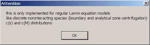
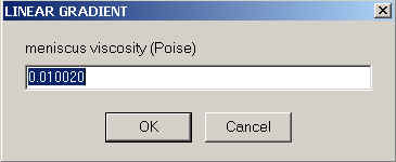
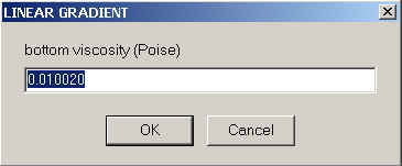
The required inputs for Sedfit are comparatively simple - we need to specify the viscosity at the meniscus and bottom,
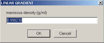
and for the density at the meniscus and bottom
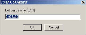
The local density and viscosity at any point in the solution column will then simply be a linear interpolation between these extremes.
A warning will appear that the macromolecule is assumed to be incompressible,
and the standard inputs for partial-specific volume of the macromolecule
and the option to optimize it's value will appear.
Constant Solvent (with solvent corrections)
The constant solvent mode is even simpler - there's no gradient at all. Nevertheless, it has been incorporated to check the algorithms and transformations for consistency. It could also be used routinely to use Sedfit in a way to produce results in corrected s-values instead of experimental ones. However, I would advise against this and instead recommend SedPHAT for that purpose (if required). The constant solvent mode is limited to work with non-interacting and concentration-independent sedimentation, only (also excluding ls-g*(s)).
The required inputs for Sedfit are like the linear gradient mode, only there's a single viscosity and density value throughout. Everything else is the same (in fact, for debugging purposes, it was built internally on the linear gradient model, setting the meniscus and bottom solution properties to be identical).