A detailed introduction of the principle of regularization, the maximum entropy method, the differences between maximum entropy and Tikhonov-Phillips regularization and other topics are presented in the size-distribution tutorial.
Prior Knowledge of Discrete Species
use c(s) integration ranges from file
Transform differential to integral distribution
Transform g(s*) to direct boundary model
suppress baseline correlation in Max Ent
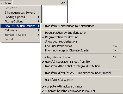
Options | Size-Distribution Options | Transform s-Distribution to r-Distribution
This function allows several transformations of a previously calculated sedimentation coefficient distribution (e.g. obtained from ls-g*(s)). These can only be calculated in sequence:
1) s(app) into s(20) [this can be done separately with the calculator function]
2) c(s20) into a distribution of hydrodynamic radii c(R). (since s~r^2, a correction factor of 2r will be inserted for transformation of the integral ds into dr) [this transformation from Stokes radii to s-values can be done separately using a calculator function]
3) corrections for a radius-dependent signal contribution (such as caused by Mie scattering).
For the correction of the signal, a file with the signal as a function of hydrodynamic radius must be provided, expressed in a power-series
signal(r) = a0 + a1*r + a2*r^2 + a3*r^3 + ... (with r in units of nm)
The format of the file should be a simple list of coefficients:
a0
a1
a2
with as many lines (and numbers) as coefficients to be taken into account. The distribution c(R) will be divided by this function signal(r), to give relative concentrations as a function of Stokes-radius R.
Tikhonov-Phillips regularization using 2nd derivative
Options | Size-Distribution Options | Regularization by Tikhonov-Phillips 2nd derivative
The details of this technique are also outlined in the introduction to size-distributions. In brief, in contrast to maximum entropy, the Tikhonov-Phillips method implemented here uses a second-derivative operator for regularization.
![]()
This represents a constrained fit, where the first term represents the unconstrained fit with a distribution, e.g. c(M), and the second term is the second derivative constraint. The constraint is controlled by the parameter a, which can be adjusted with the use of F-statistics. The use of this constraint allows one to select the smoothest distribution of all distributions that lead to a fit that is statistically indistinguishable from the unconstrained case. This strategy is frequently used to suppress noise in the inversion of Fredholm integral equations, using a priori information that the sought distribution is smooth. Please note the difference between smoothing and regularization.
This prior knowledge of smoothness of the distribution can be well justified for g*(s) distributions because of the broadening of the ‘true’ sedimentation coefficient distribution g(s) via diffusion. This diffusional broadening can be imagined as a convolution of the true distribution by a Gaussian. Therefore, we know that this apparent sedimentation coefficient distribution must be smooth, because Gaussian-shaped for a single species, or a superposition of Gaussians for several species.
Please Note
: This regularization seems to work better with ls-g*(s) than the maximum entropy regularization. Therefore, this option is switched on when using the ls-g*(s) model.
Regularization by maximum entropy principle
Options | Size-Distribution Options | Regularization by Maximum Entropy
In brief, the maximum entropy principle can be used for regularization of a distribution analysis by executing a constrained fit:
![]()
The first term represents the unconstrained linear Lamm equation fit with a distribution, e.g. c(M), and the second term is the maximum entropy constraint. The constraint is controlled by the parameter a, which can be adjusted with the use of F-statistics.
The specific form of the maximum entropy functional is derived from the statistical (Bayesian) consideration that in the absence of any prior knowledge on the distribution c(M), all the M values are a priori equally probable. The form clog(c) can be shown by combinatorial methods to be proportional to the number of microstates that can form the macroscopic distribution c(M). This can also be related to the informational entropy introduced by Shannon. For a more complete description, see the introduction to size-distributions, or, e.g. Press et al. Numerical Recipes in C.
The use of the maximum entropy functional as a constraint allows one to calculate the distribution (e.g. c(M) or c(s)) that fits the data well (statistically indistinguishable from the unconstrained case), but provides only the minimal information required to fit the data. In other words, this allows us to deviate only as little as possible from the underlying principle of not giving any preference to any particular value of M, and in this way extract only the essence of the data.
In practice such regularization is often used for suppressing noise amplification in the inversion of Fredholm integral equations.
Please Note
: Maximum entropy helps suppress artificial oscillation in the derived size-distributions. In my hands, it worked better than the Tikhonov-Phillips second derivative regularization when using the continuous Lamm equation model. However, for regularizing the least-squares g*(s), the Tikhonov-Phillips seems to work better.
Options | Size-Distribution Options | Show both regularizations
When this function is switched on, both maximum entropy and Tikhonov Philips regularizations will be displayed. This setting can be saved in the startup preferences. When copying the distribution to the clipboard, the user has to specify which trace to copy.
Options | Size-Distribution Options | Use Prior Probabilities
(keyboard shortcut: control-W)
This functions allows to switch on or off the use of Bayesian prior expectations for weighting the regularization. This can lead to strong enhancement of resolution. The general concept and the detailed implementation is described in
P.H. Brown, A. Balbo, P. Schuck (2007) Using prior knowledge in the determination of macromolecular size-distributions by analytical ultracentrifugation. Biomacromolecules 8 (2007) 2011-2024
which the user is strongly recommended to read before using this function. The following just describes the input parameters:
 '
'
The top left checkbox switches the use of prior expectation on or off. There are currently three types of prior implemented:
1) From File: This allows to use a two-column ASCII file specifying the probability distribution. The format is the same as the format generated when saving sedimentation coefficient distributions. The checkbox "GJT" file indicates a different format: that generated when saving Gilbert-Jenkins boundary shapes in SEDPHAT. Regarding the terminology, it is recommended to address this c(s) as c(P)(s).
2) Select Peaks from Current Distribution: This is the same as the keyboard shortcut control-X. This is an implementation of the idea that all species should be delta-peaks (e.g., for mixtures of pure proteins each with a single conformation and no microheterogeneity). From an existing c(s) distribution, the peaks are automatically detected. For each, a (numerical representation of a) delta-peak is placed at the weight-average s-value integrated across the peak. Note - for this, a conventional c(s) analysis needs to be performed first before using this option. It is suggested to refer to this c(s) version as c(Pd)(s)
3) From Gauss/Delta-Peaks: This allows the user to manually specify several peaks to put emphasis at the indicated locations. When the width parameter is set zero, a delta-function is used. The amplitude is governing the area of the Gaussian. Typically useful values have been between 1 and 1000, but other positive values can be used, as well. (Amplitudes of zero switch the Prior off.) Note that the Gaussian is calculated on the grid of s-values, which can distort the Gaussian substantially if the width is on the same scale or smaller than the distance between neighboring s-values in the distribution. Again, for clarity it is recommended to refer to this c(s) as c(P)(s).
When running Bayesian analyses, make sure that
1) Use Prior is selected.
2) either one of the types of prior is selected.
The prior is then shown as red dashed line in the distribution window.
After the prior expectation has been specified, do a RUN command to use the prior in the calculation of the distribution.
When using the prior for the c(s,ff0) distribution, after closing the input box shown above, you will get a chance to input separately the prior in the f/f0- dimension. You'll be asked the same information about location, width, and amplitude of expected f/f0 values. When you're done enter a value of 0. If you don't want any prior in the f/f0 dimension, then say YES to the question "do you want to use the prior", but then enter 0 for the first f/f0 value.
Prior Knowledge of Discrete Species
Options | Size-Distribution Options | Prior Knowledge of Discrete Species
this is a shortcut for the execution of the above command switching on the Bayesian modeling with the option "Select Peaks from Current Distribution", followed by a RUN command. This permits the simplified workflow:
1) calculate a normal c(s) distribution
2) use control-X to calculate the c(s) with the expectation that all peaks should be sharp. It should be useful, for example, for mixtures of pure proteins each with a single conformation and no microheterogeneity.
3) inspect the areas of the resulting peaks: a notepad file will pop up that shows how much material is unaccounted for by the discrete peaks. As described in
P.H. Brown, A. Balbo, P. Schuck (2007) Using prior knowledge in the determination of macromolecular size-distributions by analytical ultracentrifugation. Biomacromolecules 8 (2007) 2011-2024
this can be an indication that the expectation of truly monodisperse material in each peak is not sufficient to explain the data: either previously unresolved smaller peaks exist (as shown by the distribution now obtained, with the amounts indicated), or the underlying assumption is not true.
Note that the Bayesian analysis can only give you different distributions that fit the data equally well. Which of the distributions is more likely the true one depends on the reliability of the prior that was supplied to the analysis. In any case, however, the Bayesian analysis lets us explore the range of possible distributions that fit the data equally well.
Options | Size-Distribution Options | Integrate
This function allows integration of the distribution over a specified range. This can be useful to measure the fraction of material sedimenting with a given s-value (e.g., the area of a peak), as well as the weight-average s-value of this material.
Please note: Starting from version 8.5, this integration function has the keyboard shortcut ctrl-i
First, the range needs to be specified. A message box will appear that reminds that this function works exactly as the zooming tool for the distribution plot:

For that, the mouse will change into a crosshair, and the user is expected to draw a rectangle covering the desired range of s-values (or M-values, respectively) while the right mouse button is pressed. This works in exactly the same way as the rescaling function for the distribution plot (for an example of the rescaling function, follow this link).
The y-value of the rectangle is irrelevant. In our BSA example, if we want to analyze the ~6.7S peak, we can specify the range with this rectangle:

Releasing the right mouse button after spanning the rectangle will immediately display the information

on the integration range, the loading concentration (0.25 fringes) of the material under the specified peak and it's fraction of the total loading concentration (3.8%), as well as the weight-average s-value of the material, which is 6.68S.
It should be noted, however, that the fraction of the total material (the 3.8%) does include all peak, including the artificial ones at small s-values! In order to get the true fraction of the sedimenting material, we need to integrate over the range of sedimenting material, and calculate the fractions of the individual peaks appropriately.
An example of the usage of the integration tool is shown here.
New in version 8.7: An additional output is added to the integration result message: the square root of the second central moment of the distribution in the selected range. This is essentially the standard deviation, which can be used as a measure for the spread of the distribution. This can be useful measure to distinguish different samples, provided the data are acquired under similar conditions. Please note that the spread will be governed not only by the polydispersity of the macromolecular sample, but also by the regularization procedure (i.e. the P-value used, the signal-to-noise ratio of the data, number of data points, etc.) - see the size-distribution tutorial.
New in version 9.3: The result of the integration will automatically be added into the clipboard.
use c(s) integration ranges from file
Options | Size-Distribution Options | use c(s) integration ranges from file
This option allows to automatically apply multiple, pre-defined integration limits. Instead of drawing an integration range with the mouse, when this option is switched on (it can be made the default), the integration limits are taken from a specified file. The format of this file is a two-column ASCII, with tab or empty space separation.
The file (default extension *.dat) is specified when switching the option on. To change the file, you have to switch the option off, first, and then on again.
For example, the file
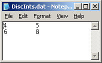
will produce, after integration is invoked, the output

The numbers are automatically silently put into the clipboard, as well, ready for pasting into a spreadsheet program.
Transform Differential to Integral Distribution
Options | Size-Distribution Options | transform differential to integral distribution
This function integrates the differential size-distributions (e.g. c(s)) and generates an integral distribution (denoted here as C(s)), following the equation

This can sometimes be useful for comparison with other integral distributions. By design, the integral distribution is scaled to the total loading concentration, i.e. C(s-max) = ctot.
Back-transform g(s*) to direct boundary model
Options | Size-Distribution Options | transform g(s*) (as ASCII) to direct boundary model
The current implementations of the dc/dt method to calculate g(s*) are algorithms to transform and average experimental data into the space of apparent sedimentation coefficients, producing the distribution g(s*). One drawback of this approach is that there is no control how well the transformed data still represent the experimental data. From the framework of the ls-g*(s) distribution, however, it is quite straightforward to build a boundary model from the g(s*) distribution by piecing together the step-functions corresponding to each s* value. After the macromolecular sedimentation boundaries corresponding to g(s*) have been reconstructed this way, the time-invariant noise and/or radial-invariant noise components can be calculated algebraically (restoring the degrees of freedom eliminated in the time-derivative dc/dt).
As a result, you can compare if the g(s*) distribution is a realistic representation of the data or not. You will get an rms error of the g(s*) model, which may be used, for example, as a direct and rational criterion if too many scans were used in dcdt or not.
This approach and the results are described in detail in Analytical Biochemistry 320:104-124.
Instructions for use of this model are simple (a reminder will be given when using it): After calculating g(s*) by dcdt (for example using DCDT+), write the distribution data to an ASCII file with error estimates, and then select this file in sedfit. Note that you should not correct the s-values to s20,w - you need to use uncorrected s-values.
Options | Size-Distribution Options | transform c(s) to c(M)
This is a quick way to get from c(s) to c(M) without changing the model. It includes the proper renormalization (M-distributions are shown on a M^(2/3) power grid) that usually requires re-running if one changes the model from c(s) to c(M).
Options | Size-Distribution Options | compute with multiple threads
Many computers now have processors with multiple cores, i.e. they are able to run multiple jobs concurrently. This can speed things up significantly. When this option is switched on, SEDFIT can make use of that for the most time-consuming step of calculating normal equations (and this will be further exploited in the future for other features).
When invoking this menu function, a message appears:

To switch this on, click on 'yes' . Then enter the number of computing cores available on your computer (or the number you want to use)

If you are not sure how many processor cores you have, right-click your mouse on the Windows taskbar and invoke the Task Manager. Select the Performance tab and you will see a picture of the current CPU usage. Note that the CPU Usage History field may have multiple small graphs. The number of graphs in this field is the number of cores you have.

In this case, the number is 8 (on a dual-processor quad-core workstation).
suppress baseline correlation in Max Ent
Options | Size-Distribution Options | suppress baseline correlation in Max Ent
When using the standard maximum entropy regularization for data that do not allow to distinguish well the baseline from the signal in the smallest s-value of the distribution, it used to be that the resulting baseline correlation can create a large increasing signal in the distribution. When the present option is toggled on, this correlation is suppressed by using the Bayesian expectation that the signal at s-min should vanish if possible. If the resulting distribution still shows a half-peak at the lowest s-value it means that there really is sedimenting material present, and one may want to lower the s-min value to get a better description of that material.