
a
M(s) for spherical or asymmetric particle
calculate weight average s by second moment integration
calculate hydrodynamic friction force
molar mass for a particle at given s-value
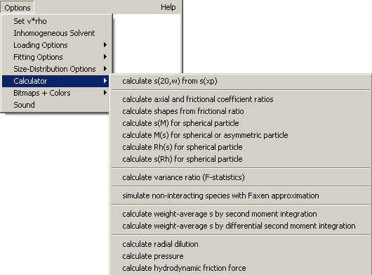
Options | Calculator | Calculate s(20,w) from s(xp)
All functions in SEDFIT (except for the inhomogeneous density gradient models) will provide s-values in experimental conditions. Since for some models, like c(s), the buffer viscosity, density, and macromolecular partial-specific volume is entered anyway (to scale f/f0 to a meaningful quantity), these entries can be used in this function to convert the experimental s-value into a value under standard conditions (water 20C).
This will transform the sedimentation coefficient distribution from experimental to standard conditions (water at 20C). The reason why this is not done by default is that for mixtures of different components it is frequently not possible to find a common value for the partial-specific volume. This will affect the spacing in s(20,w) between different peaks containing different components.
Calculate axial and frictional coefficient ratios
Options | Calculator | Calculate Axial and Frictional Coefficient Ratios
For calculation of axial ratios of elliptical shape models, once the Lamm equation modeling has revealed s and M. (For calculating axial ratios from f/f0 from using c(s), see next function below). This functionality is similar to that of sednterp, but for convenience included here. The calculations are based on the formulas from Sednterp.
Input:
1) the molar mass of the species
2) its sedimentation coefficient
3) the partial-specific volume (this function does not account for hydration)
4) the hydration
5) the temperature of the run - please note: (this is for RT - factor in the Svedberg equation, not for any temperature correction of v-bar or the viscosity)
6) the buffer density
7) the (absolute) viscosity of the buffer - please note: input is required here in Poise (i.e. 0.01002 for water at standard conditions) as is the output from sednterp.
Output:
1) a summary of the conditions specified
2) the hydrodynamic radius of the species
3) the diffusion coefficient
4) the frictional coefficient ratio
5) axial ratios for oblate and prolate ellipsoid models that would have the same frictional coefficient ratio
Calculate shapes from frictional ratio
Options | Calculator | Calculate Shapes from Frictional Ratio
This closely related to the function above, except that you don't specify s and M, but instead use directly a known frictional ratio (default is the current value of c(s)), together with the partial-specific volume, and an estimate for hydration. This result in prolate and oblate axial ratios.
Calculate s(M) for spherical particle
Options | Calculator | Calculate s(M) for Spherical Particle
Calculates the expected sedimentation coefficient for a spherical particle of the given molar mass. This does not take into account the hydration.
Input required:
1) the molar mass of the species in Da
2) its partial specific volume in ml/g
3) the temperature of the hypothetical experiment - please note: (this is for the RT - factor in the Svedberg equation, and does not take into account any temperature correction of v-bar or the viscosity)
4) the buffer density
5) the (absolute) viscosity of the buffer - please note: input is required here in Poise (i.e. 0.01002 Poise for water at standard conditions) as is the output from sednterp.
Output:
1) a summary of the conditions specified
2) the calculated s-value for a spherical particle (without hydration!)
3) the hydrodynamic radius of the sphere
4) the diffusion coefficient.
The calculations are based on the formulas used in Sednterp.
Calculate M(s) for spherical or asymmetric particle
Options | Calculator | Calculate M(s) for spherical or asymmetric particle
Calculates the molar mass that belongs to a certain sedimentation coefficient, given a certain frictional ratio.
Input required:
1) s-value
2) hydrated frictional ratio
other parameters, such as temperature, buffer density, viscosity, and vbar are as specificed in the c(s) parameter input box.
Options | Calculator | Calculate Rh(s) for spherical particle
Calculates the s-value that would be expected for a particle of given Stokes radius under the specified experimental conditions.
Options | Calculator | Calculate s(Rh) for spherical
Calculates the Stokes radius that would correspond to the observed s-value of a particle sedimenting under the specified experimental conditions.
Options | Calculator | Calculate Variance Ratio (F-Statistics)
For statistically comparing the quality of two fits, this function allows to calculate the variance (or sum of squares) increase that is associated with a given confidence level, for a given number of degrees of freedom. This is done using the F-statistics (please see this page for more information on the distribution). The calculator is used in the example for using Sedfit for testing the significance of a contaminating species, and the confidence limit of an s-value.
It is useful when we want to compare two fits, both dealing with a certain number of data points (n1, and n2), and both with a number of fitted parameters p1 and p2.
For this calculator function, information required is the following:
1) the desired confidence level (e.g. 68% for one standard deviation, or 95% for higher confidence)
2) the 'first degree of freedom' - this is in general the total number of data points considered in the fit minus the number of fitting parameters, i.e. n1 minus p1
3) the 'second degree of freedom' - this is n2 minus p2.
(there are some finer points about degrees of freedom when additional constraints are active, such as positivity, or regularization, but when n is very large, this can in most cases be neglected)
Information output:
1) The minimal increase of the sum of squares that would be required at the given confidence limit for deciding that the two fits are different. If the sum of squares is lower than this critical value, the fits cannot be considered statistically distinguishable. For simplicity, we assume here that all data points have the same statistical weight (which is a very good assumption for the interference data).
2) The rmsd that this sum of squares ratio would correspond to, for the given fit.
Please Note
: The increase in the sum of squares should not be mistaken for the increase in the rmsd of the fit. If the comparison of the fits is made on the basis of the rmsd ratio, then the square root of the critical value given by this routine has to be taken as the cutoff value.See also: F-statistics, calculation of confidence intervals, and error contour maps
Options | Calculator | Simulate non-interacting species with Faxén solution
This function allows to calculate the Faxén solutions of the Lamm equation

It can only be used if the model for non-interacting discrete species is switched selected. Invoking this function executes one simulation, but replacing the finite element solutions of the Lamm equation with the Faxén solutions. The purpose of this is only to study and compare different Lamm equation approximations. This function should not be used to analyze data, because large errors are introduced in this approximation.
Calculate weight average s by second moment integration
Options | Calculator | Calculate weight average s by second moment integration
Options | Calculator | Calculate weight average s by differential second moment integration
This function calculates a weight-average s-value by integrating the sedimentation profiles between meniscus plateau and solution plateau (similar to Fujita, Eq 2.234, see ref Schuck, Anal. Biochem. 2003, 320:104-124). This is a completely model-free weight-average s-value, valid for interacting or non-interacting systems.
This function requires solution and solvent plateaus to be established at bottom and meniscus, respectively. Also, all systematic noise should have been eliminated. The right fitting limit (right green line) should be at a position such that a plateau exists 0.1 cm inside (i.e. left of, i.e. at radius smaller than) the green line.
Because the weight-average s-value in interacting system is a function of the plateau concentration, which will drop with time during sedimentation, the weight-average s-values can also drop with time. Although this is usually only a small effect, a table of sw-vs-c(plateau) will automatically be stored in the clipboard and can be pasted into any spreadsheet program.
Note that the baseline offsets are not taken into account in this method.
New in version 8.7: Differential second moment integration - this is based on the same concept as the second moment integration, but analyzes the rate of change of the mass of material remaining at radii smaller than the right fitting limit (rather than using the absolute values of the remaining mass in relation to the initial mass). The advantage of this method is that it is completely independent of the location of the meniscus position, and the history of the sedimentation experiment prior to the scans considered. This makes it the only rigorous analysis for multi-component systems after intermittent convection. (The Lamm equation solution with an experimental scan as initial condition does also work in this case, but only for single species or for self-associating single-component systems.)
Options | Calculator | Calculate radial dilution
For the sedimentation times and rotor speed as determined by the currently loaded data, and for a species sedimentation with an s-value that can be specified, this function calculates the hypothetical position of a non-diffusion particle, its % radial dilution in the last scan, and the (time) average radial dilution the particle has suffered from time 0 to the time of the last scan. It also gives the average plateau concentration (radial dilution) in all scans.
Options | Calculator | Calculate pressure
Since it might be useful when considering pressure effects, this function calculates the pressure at the bottom and in the middle of the cell (given the currently loaded data set). It also uses the current setting for the buffer density.
Calculate hydrodynamic friction force
Options | Calculator | calculate hydrodynamic friction force
Sometimes it is worth considering the actual frictional force on the sedimenting molecule. This can be calculated using the formulas
f = 6*pi*viscosity*StokesRadius
F(friction) = v*f
s = v/(omega^2*r)
[with linear velocity v, friction coefficient f]. This function will calculate the force, given M, s, radius position, and buffer conditions.