This menu contains the following options for fitting:
* set fitting limits for meniscus and bottom
* change fit updating preferences
Options | Fitting Options | Fit M and s
This toggles the use of M and s (default) or of D and s as independent parameters to be fitted for each of the solutes. Both treatments are equivalent and related through the Svedberg equation:
![]()
Dependent on what is chosen, the parameter dialog box will show either M or D, and values are being transformed accordingly. If the checkmark is visible, M and s are in use. If no data are loaded when switching, the transformation will assume 20C as sample temperature, until this value is overwritten by loading data.
Please note: if the molar mass is chosen as parameter, the partial specific volume must be specified. Either it should be set to the correct value, or it should be set to zero (making the molar mass to the buoyant molar mass M(1-v-bar*rho). Because the diffusion coefficient is the primary measured quantity, the partial-specific volume is irrelevant.
When the parameters are switched from (s,M) to (s,D) or vice versa, M or D, respectively, are calculated for each species using the current setting of the s-value of the particular species, and of the partial-specific volume and buffer density.
Using M as the boundary spreading parameter can allow input of the frequently known molar mass, or simpler interpretation of oligomeric stoichiometry, and this setting is therefore the default. On the other hand, the diffusion coefficients may be known from dynamic light scattering experiments.
Constraints for Fitting of Meniscus and Bottom
Options | Fitting Options | Set fit limits for meniscus and bottom
If the meniscus or bottom position is treated as a floating parameter to be optimized (see parameters), it can be very useful to introduce constraints (i.e. limits) for these parameter values. For example, while the precise position of the ends of the solution columns may not be visible due to optical artifacts, the boundaries of these optical artifacts in general represent limits for the possible positions of the bottom.
Always when checking the meniscus or bottom the first time, this menu function is automatically invoked to remind the user of the importance of entering reasonable limits for these parameters. With this menu function, these limits can be changed.
TIP: If intensity data are collected instead of absorbance data, the bottom position is easier to specify. Once the intensity data have been inspected, they can be transformed to conventional absorbance data using the loading option for transforming intensity to absorbance files.
Options | Fitting Options | Lamm equation parameters
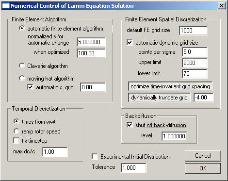
Don't panic! This is a control box that is not usually needed since the default values automatically adjust the Lamm equation parameters to what's best. The box here is just providing opportunities to explore the different numerical methods. Rarely is it necessary to fine-tune numerical parameters to better perform for extreme sedimentation conditions.
All numerical details are published in
*
P.H. Brown, P. Schuck (2007) A
new adaptive grid-size algorithm for the simulation of sedimentation velocity
profiles in analytical ultracentrifugation.
Computer Physics
Communications in press
* P.H. Brown, P. Schuck
(2006) Macromolecular size-and-shape distributions by sedimentation velocity
analytical ultracentrifugation.
Biophysical Journal 90:4651-4661
* J. Dam, C.A. Velikovsky, R.A. Mariuzza, C. Urbanke, P. Schuck (2005) Sedimentation velocity analysis of heterogeneous protein-protein interactions: Lamm equation modeling and sedimentation coefficient distributions c(s). Biophysical Journal 89:619-634
* P. Schuck (1998) Sedimentation analysis of non-interacting and self-associating solutes using numerical solutions to the Lamm equation. Biophysical Journal 75:1503-1512.
* P. Schuck, C.E. McPhee, and G.J. Howlett. (1998) Determination of sedimentation coefficients for small peptides. Biophysical Journal 74:466-474.
* J. Dam, P. Schuck (2004) Calculating sedimentation coefficient distributions by direct modeling of sedimentation velocity concentration profiles. Methods in Enzymology 384:185-212
There are four major parameter sets:
and the remaining parameters
This largely reflects parameters that are important only when not using the spatially optimized finite element discretization.
The moving frame of reference method for solving the Lamm equation is highly recommended for simulations at high ratio w2s/D, i.e. for the fitting of data sets that exhibit a relative clear and steep sedimentation boundary. On the other hand, for small sedimentation coefficients or simulations of the approach to equilibrium the Claverie method is advantageous because it allows the use of an adaptive time increment, which can be made very large for slow sedimentation processes (see the introduction to Lamm equation solutions). In order to simplify the use of the program, if the checkbox auto method is checked, the algorithms can be automatically switched, according to s-value of the simulation. This option is on by default.
The present menu function allows the user to specify the sedimentation coefficient at which the algorithms are changed (Claverie below the specified value, moving hat above the specified value). The default value is 5. The actual s-value that is used for changing the method is corrected for different rotor speeds by the factor (w /30000)^2. It may be useful to change this value if, for example, during the fitting procedure error messages show up prompting the user to increase the discretization grid size (an error message from the Claverie procedure, if negative concentrations occur due to too coarse grids or time-steps). Also, this setting might be changed to a higher value if the Lamm equation distributions are initially very slow. In the context of the optimized Lamm equation spatial discretization, the switchover can be done at much higher s-values.
The field "automatic s_grid" by default is on: when using the moving hat algorithm this adjusts automatically the movement of the frame of reference to the sedimentation coefficient of the simulated solute. This will reduce the simulation on the moving frame of reference to diffusion and radial dilution. This algorithm also works automatically with a fixed time-step, which is determined by the movement of the frame of reference. This size of the time-step, however, can be constrained to smaller values (not to larger ones).
2) Finite Element Spatial Discretization:
The "default FE grid size" determines the number of radial increments (dividing the solution column from meniscus to bottom) on which the numerical solution of the Lamm equation is based. Usually, ~ 100 per mm solution column is a reasonable value. Higher accuracy of the Lamm equation solution can be achieved with higher values, but generally the experimental noise is much larger than the error at a discretization of 100/mm. Coarser grids are faster for simulation, but less precise. For complicated situations with time-consuming Lamm simulations, it can be a good strategy to use a coarse grid to get the floating parameter values in a good range, and to use a very high number of grid points only in the end as a final refinement step.
The "automatic dynamic grid size" checkbox allows the setting of the grid size to be automatically adjusted, dependent on s- and D-values, such that a preset precision of the Lamm equation solution will be achieved.
P.H. Brown, P. Schuck (2007) A new adaptive grid-size algorithm for the simulation of sedimentation velocity profiles in analytical ultracentrifugation. Computer Physics Communications in press
As described in the paper, accuracy better than 0.001 can be accomplished with a "alpha" value of 5 points per sigma. Larger values produces finer grids with more precise Lamm equation solutions. There are upper and lower limits for the grid size that is going to be used.
This switch allows to calculate the time of scan after start of the centrifuge from the w2t entry of the file (on, is default), instead of taking it from the t entry. The advantage of this is that the time needed for acceleration of the rotor, while the centrifugal field is not fully established yet, is not weighted as much. The status of this switch is indicated by the checkmark.
An alternative method, the incorporation of the rotor acceleration phase into the Lamm equation solution is a little more precise, and recommended for larger particles, or if less than the maximum acceleration at the XLA is used.
Please Note: The
w2t entry of the centrifuge file format has a limited precision. The errors introduced by this in the calculated elapsed seconds can be observed if data are simulated, saved, and re-analyzed. For real data, however, this error will be insignificant.Simulate Rotor Acceleration Phase
The entries in the file headers saved by the XLA/XLI contains both a w2t entry (the integral over w2dt) and an elapsed seconds entry. From the combination of known rotor speed, the elapsed seconds, and the elapsed w2t can be calculated how long it took to bring the rotor to speed (assuming a linear acceleration). This is being calculated when loading files:
If the rotor gets within the time ts to the final rotor speed w0 by constant acceleration dw/dt, the integral over w2dt will have the value
once it is at speed. Therefore, the difference between the real w2dt (as read from the data file) and the w02dt of an 'ideal' experiment with instantaneous acceleration is 2/3 x w02ts . Since we know the time of the scans t, as well as the real w2dt and the rotor speed w0, we can calculate the acceleration time as
The acceleration follows as dw/dt = w0/ts. With maximum acceleration setting on the Optima XLA/I, this value is usually around 200 rpm/sec.
If the option ‘ramp rotor speed’ is toggled on (it will then have a checkmark), the acceleration phase is incorporated into the finite element solutions of the Lamm equation. Technically, this is done by discretizing the time, and recalculating after small intervals the matrix intervals related to the rotor speed.
In theory, ramping the rotor speed for the Lamm equation solution is the most precise way to deal with the rotor acceleration, since it can correctly account for both diffusion and sedimentation in this phase.
Please Note
: Information about the state of this switch is not being stored in the information on the previous best-fit. Therefore, when reloading analyses from the hard drive, this feature will not automatically be switched to its original state .fixed dt is a checkbox that can be used to constrain the time-step size. The effective value (in sec) will be the one entered in the field ‘max dc/c (or dt)’.
max dc/c (or dt) has two different functions, dependent on which Lamm simulation algorithm is chosen. In a stationary frame of reference (Claverie simulations), an adaptive time-step driver is used. In this case, the max dc/c parameter refers to the maximum change in any of the concentration values that is desired, and according to which the size of the time-step is adjusted. A larger value of max dc/c effectively increases the time-steps, while a smaller value decreases the time-steps. The detailed algorithm used is slightly more complex, and also depends on the steepness of the simulated boundary.
! If the desired relative change max dc/c leads to too large time-steps, it is automatically reduced.
For the moving frame of reference simulation, this field has no direct function. However, if a fixed dt is chosen, the time-steps in both the Claverie and moving hat algorithm are constrained to the value given in this field (in seconds).
In many cases, the back-diffusion part of the sedimentation experiment is not of interest. This is true, in particular, for large species, where the gradients become very large, and localized to the bottom of the cell. This raises the following points:
* the large concentration gradients may cause aggregation of the soluble macromolecules and/or phase transition into a surface film, both of which are processes we do not want to deal with in the experiment
* the optical detection of large gradients is not possible
* the fitting of the large gradients will be very sensitive to the bottom position of the cell, which is not directly observed and would need to be a fitting parameter, as well
* the numerical simulation of the steep concentration increase is very time-consuming and expensive.
In this case, it does not make sense to spend computational time to even model the back-diffusion part (just like we wouldn't attempt to model the formation of a surface film). Therefore, we can use Lamm equation solutions for an infinite solution column. We have published how the boundary conditions of the finite element solutions of the Lamm equation can be adapted for a permeable bottom (J. Dam, et al., Biophysical Journal 89:619-634 ).
If this option is set, this function estimates for each species the extent of back-diffusion assuming that the final equilibrium distribution has the maximal build-up of back-diffusion. At the currently set fitting limit, if the final equilibrium signal does not exceed 0.0001-fold the loading concentration, back-diffusion will be irrelevant and the Lamm equation will be solved with the permeable bottom model.
The threshold can be defined by the user, the default value is 1 (as a multiplier to the factor 0.0001).
For example, within the s-range of a c(s) distribution, some species may be small and exhibit back-diffusion, while others are so large that their back-diffusion is compressed into the (invisible) immediate vicinity of the bottom. If this function is on, the sedimentation of small species will be simulated conventionally, while the sedimentation of the larger species is simplified by using the permeable bottom model.
The assessment of the final equilibrium distribution is made using the analytical solution for ideal sedimentation equilibrium. This may somewhat underestimate the back-diffusion for strongly concentration-dependent repulsive interactions (a situation for which the threshold may be reduced). On the other hand, if aggregation and surface adsorption reduces the amount of back-diffusion, in theory, the threshold could be increased. However, these considerations are second or third-order effects, and in practice likely irrelevant.
Experimental Initial Distribution: The numerical Lamm equation solutions allow for any concentration distribution to be taken as a starting point for the simulation of the evolution. Sometimes, it can be very useful to load an experimental scan as initial distribution, for example when using boundary forming loading techniques, or when convection occurred in the initial parts of the experiment. A detailed description of this approach is given here. It should be noted that with the non-interacting species model, only a single component can be used.
Tolerance governs the Simplex non-linear regression routine: It determines the (maximum) percent change in the parameter values below which a single Simplex is stopped. The Simplex is then repeatedly restarted, until all final parameter values are within this tolerance in two sequential simplex runs. Default value is 1.
Change fit updating preferences
Options | Fitting Options | change fit updating preferences
From version 9.2 and higher, it is possible to observe the improving quality of
fit during the optimization process. This function lets you select which
graph will be dynamically updated. Considerations are the computational
cost of updating the display (dependent on the number of files and perhaps the
speed of the video output of your computer).
Note, this function is controlling cosmetic aspects only. You should not be tempted to interrupt the fit just because visually it seems to be sufficiently improved.
Also, note that the c(s) distribution during the optimization is without regularization!
Options | Fitting Options | Simplex Algorithm
This is an algorithm for optimization of the parameters during fitting that is very robust, because it does not take derivatives. Sometimes a disadvantage is that it does not very well home in to the absolute lowest point of a minimum and may wander around it without converging.
It is based on an initial randomized set of trial points around the current parameters. As a result, this method can sometimes jump out of local minimas when restarting.
see W.H. Press, S.A. Teukolsky, W.T. Vetterling, and B.P. Flannery. (1992) Numerical Recipes in C. University Press, Cambridge
Options | Fitting Options | Simulated Annealing
This is implemented similar to the Simplex algorithm, except that it does not need to go strictly downhill, at first. Only parameter values that produce fits worse than a certain threshold ('temperature') are rejected. In successive steps, the threshold is made more stringent after a certain number or trials ('annealing').
This is an excellent algorithm for optimizing many highly correlated parameters, because it permits exploration of a wide section of the parameter space and is not bound by local minimas.
The first input is the starting threshold
the default value of two is permitting an increase of the chi-square of the fit by two-fold the starting rmsd.
Next the number of 'temperature' steps needs to be entered
and then the number of iterations per step:
It is useful to append a final round of optimization with Marquardt-Levenberg (to home in on the minimum), which can be specified next:
see W.H. Press, S.A. Teukolsky, W.T. Vetterling, and B.P. Flannery. (1992) Numerical Recipes in C. University Press, Cambridge
Options | Fitting Options | Marquardt-Levenberg
This algorithm is excellent for very efficiently going downhill in the error surface, based on the slope and curvature of the error surface. A disadvantage can be its susceptibility to local minima. Note that it takes some time to build up the information on the local curvature, which will appear as if the optimization is very slow, but then it will usually proceed with excellent steps, making it overall usually the fastest algorithm.
see W.H. Press, S.A. Teukolsky, W.T. Vetterling, and B.P. Flannery. (1992) Numerical Recipes in C. University Press, Cambridge
Options | Fitting Options | Serialize Fit
This function allows the user to perform automatically a series of data analyses on many data sets. This can be, for example, different cells from the same run. This requires
* the data to be located in specific directories (or in the same directory)
* all analyses are using the same model
* the desired model must be currently selected
* fitting limits must be the same (e.g. when analyzing samples of similar volume)
Each data set will be fitted, and optionally a series of integrations will be performed on distributions. In the end, results are stored in the directory of the original data:
1) ~tmppars.* files: when loading the data, say YES to reload previous analysis -> this will hold the results of the serialized analysis
2) SEDPHAT configuration files: For each analysis, the best-fit model will be exported to SEDPHAT (such that the best-fit model can be retrieved by double-clicking on the *.sedphat file)
3) files "distribution.*", "ff0.*" and "integrals.*", which contain the information on the best-fit distribution, the f/f0 value, and the integration results.
When using this function, a number of boxes come up:
If you are analyzing a series of cells, with cell numbers *.ip1, *.ip2, *.ip3, etc., select YES.
You can automate the analysis of data from cells with the same cell number, if the data are located in specific locations, with the highest subdirectory being a number. Then, data can be drawn sequentially from different subdirectories.
For example,
c:\aucdata\mysample\1\00001.r01...
c:\aucdata\mysample\2\00001.r01...
You will have to generate this directory structure and copy the data into these folders. Note that the subdirectory numbers must be sequential.
If you want to analyze data only from a single run, select NO.
If you answered previously to analyze a series of cells, a question comes
For example, if the first cell is cell2 (e.g., *.ip2 data), enter "2"

Similarly, the number of the last cell to be analyzed must be entered, e.g. "7". In this example, cell 2, 3, 4, 5, 6, and 7 will be analyzed sequentially.
If you have previously selected to draw data from different subdirectories, the question
will ask for the lowest number of the subdirectory you want to analyze. This is followed by the number of the highest subdirectory
(If you didn't select this option, these boxes will not appear.)
The next question is
Generally, you'd want to select YES (unless you've already fitted previously). In this case, you can select to restore the previous fits by selecting YES to the question
Otherwise, select NO (i.e. start the analysis from scratch for each data set).
If your current model is a continuous distribution, you can automatically integrate
by selecting YES.
If you do so, the integration range will be requested:

(e.g., in this example the distribution from 0.5 S to 8 S will be integrated).
You can chose an additional integration range by selecting YES.
After this, SEDFIT will go through all the specified data sets, does the fits, and stores the results in the files (see above).