back to the tutorial main page

The use of the apparent sedimentation coefficient distribution ls-g*(s)

For preparation of this topic, please read the tutorial on ls-g*(s).

Although the c(s) distribution has big advantages in resolution over the apparent sedimentation coefficient distribution g*(s), there are situations where the deconvolution of diffusion is not desired or necessary (e.g. when working with very large particles where diffusion is negligible, or just as comparison to the results of the dcdt analysis).  It should be noted that because ls-g*(s) is a direct boundary model, we do not need to constrain the data set as much as in the dcdt transformation.  There is no broadening from too many scans.  Details are described in this reference.  However, the number of scans included should not be so large as to lead to a bad fit. 

(Please note that ls-g*(s) should not be applied to small sets of interference scans where the boundary has not yet cleared the meniscus, because of correlations of the small s-values with the unknown time-invariant baseline.) 

Sedfit has implemented the g*(s) in the form of a least-squares direct boundary model ls-g*(s).  This is described in the introduction to ls-g*(s), serves as an example in the introduction to size-distributions, and in the help-page for ls-g*(s).  Here, we only describe its practical application to the BSA data set. Another application can be seen in the example of using Sedfit.

NEW:  Please note the new integration tool, which allows calculating the weight-average s-value of the sedimenting species!

The application of the ls-g*(s) analysis has many similarities to the c(s) analysis, but it is much simpler because of the absence of deconvolution of diffusion and as a result it gives only much lower resolution.

Select the model

An information box will appear as a reminder that with ls-g*(s) the regularization method will be changed:

the relevance of this is described in detail in the introduction to the size-distribution -- we can accept this default setting.  Dependent on the previous parameter settings, a second message may appear

with the reminder that taking into account the acceleration phase of the rotor is not required in the g*(s) model.

We have to press the parameter menu to get to the settings:

The meaning of the parameters is the same as with the c(s) distribution above, except that there are much fewer parameters.  Basically, we need to adjust s-min and s-max to give the proper s-range (we know already that a reasonable range would be 1 to 12).  The resolution does not need to be nearly as high as in the c(s) analysis, because we will not need to describe any sharp peaks.

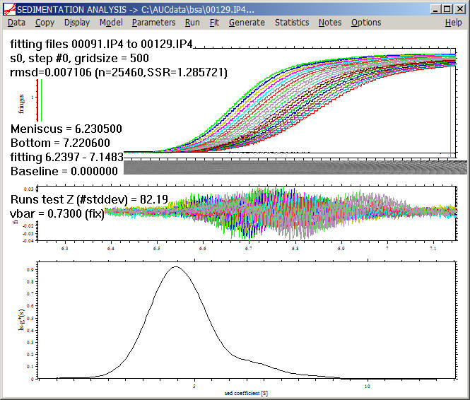
Simply executing a Run command will give us the ls-g*(s) distribution:

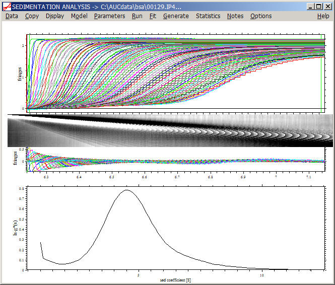
As mentioned above, the quality of the fit is in general very poor, as the apparent sedimentation coefficient distributions do not describe diffusion.  Therefore, unless we are dealing with very large particles or very high rotor speeds where diffusion is negligible, we have to reduce the number of scans in the fit to get a reliable analysis.

For example, considering only scans 90 to 129, we get a more reasonable fit if we use a high value for the 'resolution' field.  (The latter decreases the size of the step-function, and allows to differentiate the misfit due to finite discretization from misfit due to significant diffusion).

If applied to the same data subset, the result of ls-g*(s) and dcdt will be the same, with the exception if a very large data set with large Dt is used, or for very small sedimentation coefficients, where the direct boundary model ls-g*(s) is more advantageous. As described in the introduction to the size-distribution theory, due to the use of regularization there is very little noise apparent in the distribution (without smoothing). 

In some cases, it may be desirable to optimize in a non-linear regression the position of the meniscus.  One such case is when working with very large macromolecules at low rotor speed, where the deformations of the meniscus can make a graphical determination very difficult.

Note the new tool for integration of the distribution and calculating the weight-average s-value over a selected range. 

back to the tutorial main page