The example given here highlights the potential of sedimentation velocity analysis with Sedfit. Data can be downloaded, and the results can be compared with those displayed, but this will require basic familiarity with Sedfit functions as described in the step-by-step tutorial. For readers who want to get familiar with how to do these analyses, the step-by-step tutorial should be consulted first. Much more detailed introductions in the theory of the analysis techniques are available in the Sedfit help web, and will be referenced below. Similarly, references to the websites explaining the Sedfit functions applied will be given. The analysis can be refined by exporting the data and the model to Sedphat.
The data were acquired as described in the tutorial section on experimental considerations. It is a sample of IgG molecules in PBS, run at 40,000 rpm. (In principle, a higher rotor speed (55,000 rpm) could be used for studying a molecule of this size of IgG, but the main concern in this experiment was to quantify the extent of aggregation. Because possible aggregates might sediment much faster, the lower rotor speed was chosen.)
A zip archive with the data (2,541kb) can be downloaded here. In the following, for clarity we only load every third scan (of a total of 226 scans), but for a full analysis, the complete set of scans should be loaded.
After loading the data (every third of 1 - 226), we see the raw data,
which shows the typical time-invariant noise pattern, jitter, and integral fringe shifts. Sedfit will calculate these offsets by systematic noise analysis, and we do not need to do anything about that here.
(Please note the large boundary movement in this set of scans. This is useful for a high precision analysis. In fact, ls-g*(s) should not be applied to small sets of interference scans where the boundary has not yet cleared the meniscus, because of correlations of the small s-values with the unknown time-invariant baseline.)
First, we select meniscus, bottom, outer and inner fitting limit (as described here):
In this example, we might want to look first at the g*(s) distribution, to get an overview of the range of s-values. After getting used more to c(s) you probably want to move directly to the c(s) model described below. The point of this preliminary analysis is to provide a simple entry point for novices.
We might first select the ls-g*(s) model, with a range from 1 to 15 S (resolution 100, P = 0.68). After executing the Run command, this results in the following output:
It is clear that most of the material is ~ 6.5 S, with a small amount sedimenting at 9-10 S. We can subtract the systematic noise by pressing ctrl-N, which will show the sedimentation data clearer:
Please note: If the fit is bad, this reflects the diffusional fluxes which are not taken into account in the ls-g*(s) model. (This means that there is a lot more information in the data that we didn't extract yet.) At this stage, we can get a rough overview of the sedimenting species, but a serious ls-g*(s) analysis would require constraining the fit to a subset of the data. For more details, read the tutorial on ls-g*(s).
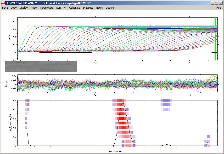
Next, we perform a c(s) size-distribution analysis with solutions of the Lamm equation, which takes diffusion into account by means of a weight-average frictional ratio. Switch to c(s) model, and enter in the parameter box a range from 0.1 to 15 S (resolution 150, P = 0.68), with an estimate for the frictional ratio of 1.5. This gives a good fit with rmsd 0.003 fringes. Subtract the systematic noise (ctrl-N), and we see this picture:
We can already see the main peak and some contaminations. The residuals bitmap,

shows a faint diagonal stripe, which indicates that it may be possible to improve the fit further.
If we expand the view
we can see some deviations in the fit of the first couple of scans:
which is the cause of the large residuals in the vicinity of the meniscus. Therefore, in a second stage, we try to refine the analysis by including the rotor acceleration in the solution of the Lamm equations, and we use the Fit command to optimize the frictional ratio and the position of the meniscus (we can temporarily switch off the regularization during fitting). Ignoring effects of partial-specific volume and solvent viscosity, this converges to a value of f/f0 of ~1.6 and a meniscus at ~ 6.071 cm**. This optimization takes between 20 and 30 min on a 900 MHz PC (it takes less time with fewer scans, e.g. every 10th). The rms error is ~ 0.0026 fringes
The residuals bitmap is now virtually free of systematic deviations:

Exporting the distribution and plotting with Origin shows more details (with break in the axis):
The s-values of the contaminating oligomeric species are slightly correlated with the f/f0 value. However, they are very significant, as well as the small fragment at ~ 0.5S. Relative concentrations can be obtained by integrating the area under the peaks.
After removing the systematic noise, we can expand the view with the mouse,
and see in lower part of the boundary close to the meniscus the presence of the small amount of low molecular weight contamination:
as well as the slight back-diffusion caused by the small molecular weight in the later scans close to the meniscus
(note the positive slope towards the bottom). Similarly, we can zoom in to the upper part of the boundary
and verify the small portion of rapidly sedimenting material in the slightly skewed shape of the shoulder. Finally, we can look at the middle part of the boundaries
and see that the diffusional spreading (decreasing slope) is well modeled.
It should be noted that the full analysis of these data will have threefold higher density of scans (left out here for clarity). This shows the level of detailed information that can be extracted from sedimentation velocity analysis by direct boundary modeling.
Switching to the c(M) distribution gives a gross estimate of molar mass distribution, which is valuable predominantly for the main species (as this governs the weight-average f/f0), less so for the oligomeric species:
NEW: The distribution plot can now be expanded in sedfit by using the new command for rescaling the distribution plot in the distribution menu. Also, using the new integration tool, we can calculate the loading concentration and weight-average s-value under each of the peaks.
After having identified the number of the components, we can now make use of our knowledge that we have actually discrete species in solution. We can switch to the non-interacting discrete species model, and use the s-values of the peaks from the c(s) analysis as starting guesses. We can fix the monomer, dimer and trimer molar masses (for simplicity approximating the effective monomer molar mass by 150kDa -- of course if known, this should be substituted by the true molar mass of the monomer, and the partial-specific volume and buffer density should be entered), and float the s-values and concentrations of all species, as well as the molar mass of the small species. For this analysis, we load the complete set of 226 scans (in this model, a large number of scans does not slow the analysis down much, as in the distribution models - although it slows down the display). Also, we include the meniscus position as a floating parameter.
[For a more general method to analyze discrete species in combination with continuous segments, or for discrete species the unknown molar masses of known oligomeric series, see the SEDPHAT hybrid discrete/continuous model].
We get the following fit, which suggests we have a total loading concentration of 0.359 fringes, and of this ~ 3% dimer, ~1% trimer, and 6% small Mw contamination.
The rms error is 0.002612 ***, very close to that of the c(s) analysis, which confirms that the peaks found in c(s) are indeed macromolecules that sediment as discrete species. Like before, the residuals bitmap shows very little systematics,
even if we use a scale of 0.01 for max black to white (instead of the default 0.05 max scale).
The remaining patterns of vertical and horizontal lines are due to small vibrations and very small drifts in the interference optics producing systematic errors that are not described by RI and TI noise, showing limitations of stability of the commercial instrument.
At this point, we could ask if the 1% trimer is really statistically significant. For this, we can use the Sedfit calculator to get from F-statistics the rmsd cutoff for the 340,000 data points that corresponds to one standard deviation (P = 0.68). We find that all fits with an rmsd higher than 0.002614 is statistically significantly worse (on a confidence level of one standard deviation). If we switch off the trimer component and refit the data, the fit converges at an rms value of 0.002686, which shows that the 1% of trimer is statistically highly significant. Note that this does not apply to the s-value, which is not well-determined, but the existence of an oligomer larger than the dimer.
The next question one might ask is what is the precision of the s-value of the main component. We use the 'confidence interval for s' function of Sedfit, which performs a series of fits constraining s1 to non-optimal values (we choose a test interval of 0.002, and a confidence level of 68%). The cutoff s-value will be reached when the rmsd of the fit is larger than 0.002614. For this analysis, we also should let the meniscus position float, as this parameter will be correlated with the sedimentation coefficients (and we don't know for sure that the previous best-fit meniscus is the true one). If the molar mass has some uncertainty, it should also been floated (for simplicity, we assume in this example that we know the molar masses of all but the small component). This takes a while because of the large number of scans and floating parameters (after a few tests to make sure everything is running OK, I did this analysis overnight). In the end, we get a confidence interval of [6.572 - 6.623] (or approximately +/- 0.026 with a slight asymmetry), which corresponds to a relative error of ~0.4%.
New in version 8.7: Please note that corrections for solvent compressibility are now available. For using those, please read the specific instructions for this Sedfit mode. They have not been included in the above tutorial, yet. For the c(s) distribution with solvent compressibility, this will mean that the s-values are corrected to standard conditions (water 20C), and that the buffer viscosity and density in the input boxes will refer to standard conditions.
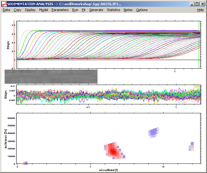
An alternative analysis for cases where we do not want to make the assumption of discrete species, we can look at the c(s,f/f0) analysis. This produces the following result:
In the absence of the knowledge of discrete species, the molar mass assignment to the trace components cannot be made, but the molar mass of the major component can be well-determined without any scale-relationship approximation:
Footnotes:
** At first, this meniscus position seems to be a little bit outside the range where it would be graphically estimated at this stage based on the appearance of the optical artifacts. However, it should be noted that after systematic noise has been subtracted, no judgment about the meniscus position can be made. If we take the best-fit meniscus position and compare it with the raw data, it does indeed look like a possible value:
Only the fact that this part of the meniscus artifact is similar in all scans has made it 'disappear' when subtracting the best-fit TI noise. In my experience, the analysis with floating meniscus yields reliable results, in particular when the data are acquired over the complete sedimentation process.
*** If the rms error is not exactly reproduced, this is due to the statistical nature of the simplex fit. However, essentially identical results should be obtained.