ls-g*(s) distribution by least-squares boundary modeling
Model | ls-g*(s)
The ls-g*(s) approach is described in the introduction to ls-g*(s). It is also part of the step-by-step practical tutorial (see the last chapter). The ls-g*(s) distribution is also used as an example in the introduction to size-distributions, from which some aspects of regularization can be learned. The application of the ls-g*(s) distribution is also shown in the example application of Sedfit. Related models are the ls-g*(s) with a superimposed diffusing species, and the extrapolation of ls-g*(s) to infinite time.
In brief, this model describes the sedimentation of a distribution of non-diffusing species. It is closely related to the results of g(s*) by dcdt, but in the form of a direct boundary model. When applied to a data set where the dcdt method is applicable (i.e. a not too much boundary displacement and a limited number of scans), ls-g*(s) and g(s*) by dcdt give the same results. However, ls-g*(s) has several advantages that make it more versatile:
1) As a direct boundary model, there is no differentiation step and no approximation of dc/dt by Dc/Dt. As a consequence, we do not need to take data from small time-intervals only. There is no extra broadening caused by having too many scans! However, a limitation in the number of scans is the requirement that the model fits the data reasonably well.
2) Ability to work with scans that have large displacement is highly useful when analyzing absorbance data, but the method works equally well for interference data, where systematic noise decomposition is used.
3) Because large boundary displacement is not an issue, experiments can be run at higher rotor speeds, which can translate to higher resolution.
4) It is suitable for combination with non-linear regression, for example for determining the exact meniscus position.
In many cases when using this model, it should be considered if the c(s) distribution is not a better way to analyze the data, because with c(s) diffusion effects are deconvoluted, giving substantially higher resolution and sensitivity. If the determination of a species molar mass is the goal, the independent species model should be used, or the hybrid discrete/continuous distribution in Sedphat .
It should be noted that SEDFIT has a model or the extrapolation of ls-g*(s) to infinite time, as a variant of the van Holde-Weischet method.
Parameters
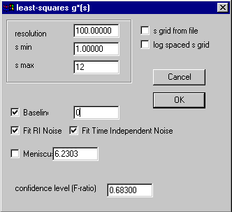
As mentioned above, the ls-g*(s) approach is described in the introduction to ls-g*(s). It is also part of the step-by-step practical tutorial (see the last chapter). The parameter box of the ls-g*(s) model is:

The meaning of the parameters is the same as with the c(s) distribution, except that there are much fewer parameters. Basically, we need to adjust the resolution, s-min and s-max to give the proper s-range. The confidence level field determines the magnitude of the regularization. The default regularization is Tikhonov-Phillips (although it can be changed), and I would recommend confidence levels of one (enter 0.68 in the confidence level field) or two (enter 0.9) standard deviations. In some cases, the distribution may have some oscillations or spikes, which can be suppressed by using higher regularization (F-ratio of 0.95 or even 0.99).
The other parameters are as usual; a floating baseline should be allowed, and when working with interference data, the time-invariant and radial-invariant noise (jitter) should also be allowed for (i.e. checked). It is possible to optimize the meniscus position in a non-linear regression; if this is desired, check the box left to the meniscus field.
Simply executing a Run command will give us the ls-g*(s) distribution in the lower plot. For optimizing the position of the meniscus, use the Fit command.
Some message boxes may appear, as described in the tutorial. As described in the tutorial, peaks at either extremes of the s-range can not be trusted, and if they occur, the range should be enlarged. Peaks at low s-values may indicate either a correlation with the baseline parameters, or that s-min should be further reduced. Peaks at s-max always indicate the presence of faster sedimenting material.
Tips:
1) For best results, it is advisable to start with a relative small range of s-values. It is recommended to increase s-max if there is an upward curvature of the distribution at the highest s-value, and conversely, to decrease the s-min value if there is a significant contribution in the distribution at this lower s-value. The problem of peaks at s-min and s-max is the same as with the c(s) distribution (described in the tutorial).
2) The distribution will automatically clipped to the maximal s-value that can be observed for the given rotor speed and time of the first scan.
3) When used in conjunction with time-invariant noise analysis, there can be a correlation of the low s-value part of the distribution with the degrees of freedom from time-invariant noise. To avoid this problem, it is recommended to use a larger data set, and scans that have cleared the meniscus.
4) increase the resolution number and check if the fit quality changes. If so, use the higher resolution setting to judge how many scans to include.
New in version 8.7: When using the inhomogeneous solvent mode, e.g. to correct for solvent compressibility, please read the specific instructions for this Sedfit mode first. For the ls-g*(s) model, this will mean that the s-values are corrected to standard conditions (water 20C).
Reference
: P. Schuck and P. Rossmanith. (2000) Determination of the sedimentation coefficient distribution g*(s) by least-squares boundary modeling. Biopolymers 54:328-341