Note, as of 2007,a significant update and improvement in the Lamm equation solution is implemented, as described in
P.H. Brown, P. Schuck (2007) A new adaptive grid-size algorithm for the simulation of sedimentation velocity profiles in analytical ultracentrifugation.
Click on this link to read how this works:
Computer Physics Communications in
press
This work is not yet included in this introductory page.
The finite difference approach and its limitation
The finite element solution by Claverie
The moving frame of reference finite element solution
The Lamm equation describes the evolution of the concentration distribution c(r,t) of a species with sedimentation coefficient s and diffusion coefficient D in a sector-shaped volume and in the centrifugal field w2r. It is a partial differential equation that, in the simplest case, takes the following form,
(1)
which can be derived from a mass conservation equation with the local diffusion fluxes D(dc/dr) and the local sedimentation fluxes csw2r.
Typical shapes of families of concentration distributions described by the Lamm equation look like this (centrifugal force pointing to the right, details would depend on the time-scale and rotor speed):
 (a)
(a) (b)
(b)
 (c)
(c) (d)
(d)
 (e)
(e) (f)
(f)
[for species with initially uniform distribution, sedimenting at different values of s and D: (a) intermediate s and D; (b) intermediate s, low D; (c) high s, low D; (d) low s, high D; (e) flotation with intermediate s and D; (f) sedimentation with intermediate s and D with initial lamellar distribution of c(r)]
Some general features can be observed:
(1) the centrifugal field causes concentration gradients (d) or sedimentation boundaries (a, b, c, e);
(2) diffusion broadens this boundary with time (visible best in a, b, e, f);
(3) radial dilution (visible best in a, b, c) or radial concentration (for floatation in e), which is caused by the sector-shaped solution column;
(4) end effects of the solution column due to accumulation of the material at one end (omitted in a, b, c, but visible in d, e) and depletion from the other end of the solution column;
(5) after a long time, an exponential equilibrium distribution is approached (visible best at low speeds or high D, such as in d)
(6) it should be noted that, although the Lamm resembles a diffusion equation, it has an extra transport term sw2r which is position dependent. It varies by about 15 - 20% for typical experimental situations.
These features make the Lamm equation difficult to solve, and eliminate the possibility of a closed analytical solution. Since it was introduced in 1929, because of the great practical importance, several approximate analytical solutions have been derived for different limiting cases (see the monograph by Fujita, 1962).
The simplest approximation is that by Faxén (1929), which can be written as
(2) 
with the meniscus position rm, the boundary position of a non-diffusing species r*(t)=rmexp(w2st) and the error function F. It has a first term describing radial dilution, a second term (1-F) for the diffusional spreading, and the movement of r*(t) describes the boundary movement. This solution describes qualitatively many features of Lamm equation solutions, in particular curves of the type in example (a). However, it is quantitatively not very precise, and it does not describe many features of the Lamm equation, such as the accumulation of material at the bottom of the cell, or the interdependence of the effects of diffusional spreading, radial dilution and the radial-dependence of the force. (Faxén solutions according to Eq. 2 can be calculated with the calculator function of Sedfit. Examples of the accuracy can be found here.)
Improved analytical solutions have been developed, including higher-order terms of analytical serial expansions, which give excellent approximations for ranges of parameter values (s, D, w) resembling many commonly encountered experimental configurations (Holladay, 1979; Behlke, 1997; Philo, 1997).
A completely different strategy for solving the Lamm equation are numerical simulations. Instead of formulating approximate analytical expressions for the concentration distribution as a function of time, the numerical simulations aim to develop computer algorithms that mimic the evolution of the concentration distribution with time. Given any distribution c(r,t), the elementary step in the numerical algorithms is the calculation of the distribution at a later time c(r,t+Dt). Many different strategies have been developed (Bethune and Kegeles, 1961, Cann and Kegeles, 1974, Claverie, et al., 1975, Cox, 1965, Dishon, et al., 1966, Marque, 1992, Minton, 1992, Sartory, et al., 1976, Schuck et al, 1998, and Schuck, 1998).
In Sedfit, numerical simulations are implemented for the following reasons:
* Although the numerical simulations may require hundreds or thousands of iteration steps, these steps can be made computationally very efficient, so that there is no relevant difference in computation speed to the approximate analytical solutions.
* The approximate analytical expressions are based on truncated serial expansions that converge best for certain ranges of parameters (s, D, w, t) or initial conditions. In fact, many of the analytical solutions are based on idealizations such as infinite solution columns. In contrast, the numerical solutions, if properly designed, are naturally very flexible to adapt much better to different parameter values and initial conditions. For example, a well-designed algorithm can give equal precision for all curves (a) to (e) shown above, as well as many other situations. It is even possible to take experimental scans as initial conditions for the simulation of the evolution in time.
* The precision is easily controlled to be well below experimental errors of data acquisition for all cases. This can be achieved by sufficient discretization in the spatial variable and adaptive step-size control in the time variable.
* Numerical solutions allow the acceleration phase of the rotor to be included in the simulation.
* They can be naturally extended to take chemical reactions and concentration-dependent sedimentation into account.
However, numerical solutions can also have drawbacks: If they are not properly designed, they may converge only very slowly to the correct solution, and exhibit spatial and temporal oscillations in the concentration distributions. Therefore, in the following the different strategies and their advantages and disadvantages are briefly described.
The finite difference approach and its limitation
The simplest way of simulating Lamm equation solutions is the division of the radial variable into a series of compartments (i = 1...N, for example with equal width Dr). Consideration of the diffusion and sedimentation fluxes between the compartments allows to predict the evolution of the concentration in each compartment.
Example for the division of a boundary (red) into a series of compartments with different concentrations (visualized as rectangular boxes of different heights).
This is inspired by compartment models as commonly used in models for chemical kinetics, and the intuitive application of compartments for the spatial discretization.
If one writes the concentrations in each compartment in vector form c(r,t), the concentration changes occurring within a small time-interval Dt can be formally expressed as
(3a) ![]() , or (3b)
, or (3b) ![]()
(with the identity matrix I and a propagation matrix E; this follows from the linearity of the Lamm equation.) If we count the fluxes going into and out of any compartment, we obtain for the discretized net diffusion fluxes -(D/Dr)[c(i+1) - 2 c(i) + c(i-1)] and for the net sedimentation fluxes w2[c(i-1)r(i-1) - c(i)r(i)]. As a consequence, one arrives at the following form of the propagation matrix E
(4) 
This is a tridiagonal system, and the evolution Eq. 3 can easily be solved for series of time-steps (Schuck et al., 1998).
One problem commonly encountered with such propagation schemes as in Eq. 3 is an oscillation caused by sequential too high and too low concentration estimates in neighboring compartments, which alternate in sign with each time-step. Once formed, such oscillations can often amplify. They can originate, for example, in regions of high concentration gradients.
![]()
A very effective way around this problem was described by Crank and Nicholson (1947). The idea is to dampen the oscillations and get higher precision of the time-steps by evaluating concentrations in the right-hand side of Eq. 3a in the middle during the time-step D t, approximated as (c(t) + c(t+Dt))/2. The physical basis for this is that as the concentrations change gradually during the time-step Dt, so do the fluxes, which are proportional to the concentrations. Although we do not calculate the exact form of these changes during the time-step Dt, it is a good assumption that the average flux during Dt is proportional to the average concentration during Dt, which we approximate by the arithmetic mean of c(t) and c(t+Dt). At first, it may seem that this is a circular argument, since we don't know c(t+Dt) yet, but a simple inspection of the equation 3a shows that in fact (c(t) + c(t+Dt))/2 can be used in place of c(t) in the right-hand side, and the resulting equation can be easily rearranged to solve for c(t+Dt) as
(5) ![]()
The Crank-Nicholson scheme gives a significant improvement in speed and accuracy of the simulation.
![]()
The finite difference approach is fast and works very well for small molecules (high D, or low rotor speeds). However, for larger s-values with smaller diffusion coefficients the approximation becomes poor, because the discretization into compartments creates an artificial diffusion term of a magnitude proportional to w2sDr , where Dr is the size of a single compartment (Schuck et al., 1998). For high D, the extra diffusion term can be neglected, but for small D it cannot, unless a very fine grid (small Dr) is used, which is very inefficient.
The origin of this error can be seen as follows: Assume the ideal linear translation of a boundary in the absence of diffusion and radial dilution, as approximated by the compartment model.
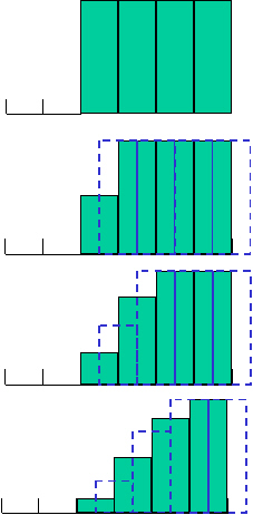 At time 0 it
may look like a perfect rectangular boundary, with empty compartments #1 and #2,
and equally filled compartments #3 to #6.
At time 0 it
may look like a perfect rectangular boundary, with empty compartments #1 and #2,
and equally filled compartments #3 to #6.
After a time-increment sufficient for the boundary to move just half the size of the compartment, Dr/2, the concentration distribution would move as indicated by the blue dashed lines. However, in our discretization scheme this means that half the concentration of each compartment flows into the right-hand neighbor compartment, and based on this we calculate the new concentrations in each compartment. Because just half the concentration is left in compartment #3, it is half the height.
After another time-increment, again half of the concentration in each compartment flows to the right - leaving 25% in #3, 75% in #4, and 100% in #5 and #6.
It can be seen that instead of translating the rectangular boundary, the compartment discretization acts like a diffusion of the boundary; the interpretation of compartments as spatial elements introduces bias in the spatial distribution.
This effect is well-known in numerical mathematics and referred to as 'numerical diffusion'. In the appropriate text-books, you can find that in order to avoid this 'numerical diffusion' the simulation may require several orders of magnitude finer grid size than the physical scales of primary interest (Durran, 1999).
In summary, the finite difference scheme is a good method for the Lamm equation only for small s and large D. The inherent problem is that the sedimentation term is not well described by the compartment model, which leads to poor convergence of this algorithm to the correct distribution, and requires very fine discretization. Although successive grid refinements can be incorporated into nonlinear regression, the finite element methods described in the following are significantly more efficient (Schuck et al., 1998).
The finite element solution by Claverie
Claverie has introduced the finite element technique to the problem of solving the Lamm equation, which is less empirically (or physically) motivated, and instead a more mathematically based approach. Nevertheless, it has many intuitive features. Instead of the approximation of the boundary by 'rectangular' compartments, the boundary is described as the mathematical sum of triangular-shaped elements called hat-functions:
(6) 
where each of the hat-function looks like, for example, the red one indicated below (triangle in left figure).
As can be easily verified, they have the property that when neighboring hat-functions added up, they describe a step-wise linear function (e.g. the red line). Eq. 6 separates the spatial and the time variable, and the problem reduces to the question of how much of each element is required to describe the boundary well at a later time (such as the reduced magnitude of the red triangle in the right figure above).
The trick of getting equations for the amplitudes ck(t) of each triangle is the multiplication of the Lamm equation with one element Pk(r) followed by integration over rdr from meniscus to bottom (equivalent to the volume integral in the sector-shaped cell). Integration by parts of the rhs can be performed, exploiting the vanishing total flux at the meniscus and bottom (Claverie, et al., 1975), and we arrive at
(7)  [for all k]
Finally, we insert our approximation Eq. 6 (renaming our running variable to j) into Eq. 7, which leads to an equation system
(8a)
 [for all k]
It should be noted that since the hat-functions Pk(r) are simple, the derivatives dPk(r)/dr are very simple, too. Also, since the spatial variable only occurs in the form of the hat functions, we can easily calculate analytically the integrals for all (j,k), and abbreviate Eq. 8a to
(8b) 
This is a linear equation system that can be easily solved. The matrices A(1), A(2) and B are tridiagonal (because the pair-wise integral over the hat-functions is only non-zero for identical or neighboring hats), and their numerical values can be found here (as C-code). Discretization of the time-variable and writing the concentrations in vector-form leads to the equation system
(9a) ![]()
or in Crank-Nicholson scheme
(9b) ![]()
This is a triangular equation system very similar to the one derived above for finite difference system, but because of the use of hat-functions instead of the compartments, it does not introduce the artificial diffusion term!
For calculating the evolution in time, Eq. 9b can be used, as long as the time-steps Dt are not too large. Initially, or when rapid changes in the concentration profiles take place, a small Dt has to be used, while near equilibrium very large Dt may be tolerable (and preferable). Therefore, to keep the discretization error small but the simulation efficient, it is very useful to adjust the size of the time-step dynamically after each step (Schuck et al., 1998).
This simulation of sedimentation works extremely well for small and medium-sized molecules; it provides a very high precision at only moderate computational cost. The algorithm has problems, however, in the case of large molecules, where the sedimentation flux is much larger than diffusion. In this case, the sedimentation boundary is very steep, and very small time-steps are required in order avoid too large changes in the ck(t) values when the boundary moves across the compartments. In fact, the algorithm is unstable for the limiting case of no diffusion (where even very small time-steps can lead to negative concentrations ck(t), followed by large oscillations). This is not very appealing, especially since there is a simple analytical solution of the Lamm equation for particles without diffusion:
(10) 
describing a rectangular step at the position rmexp(w2st) with radial dilution. This problem is solved by the moving frame of reference approach.
The moving frame of reference finite element solution
The basic idea for an algorithm that solves the Lamm equation in a stable and efficient manner for all limiting cases is the movement of all radial grid (reference) points exactly like a non-diffusing particle (Schuck, 1998). Viewed from this reference frame, there is no sedimentation visible, just diffusion, which by itself is a comparatively simple computational problem. This is similar to the idea of transformations of the radial variable that was employed for the derivation of the approximate analytical solutions of the Lamm equation (Faxén, 1929 and others, see Fujita 1962), but incorporated here in the finite element framework.
As indicated in this schematic view, in this algorithm the hat functions at the different grid points sediment with the particle, such that the relative changes in the amplitudes of our hat functions remain small, which allows higher precision and efficiency at large sedimentation flux. Mathematically, we can formulate this idea by approximating the sedimentation profiles with a linear combination of time-dependent hat functions Pk(r,t) (similar to the approximation with static hat functions in Eq. 6)
(11) 
Here, the hat functions are - like in the Claverie approach - step-wise defined triangles
(12) 
but with grid points rk that change with time as
(13) 
where the position rk(t) is that of an ideal sedimenting particle with an s-value sG . The exponential movement of the grid-points is abbreviated as a(t-t0). Only the meniscus m and bottom b are fix, since they have to denote the constant solution column position measured as distance from the center of rotation.
There is one obvious problem - how can we choose a good set of radial grid points for the entire simulation, when they permanently 'sediment' towards the bottom of the simulated centrifuge cell? The key is to use a properly spaced initial grid consistent with the movement of grid points, and then to change the grid at well-defined times. This works as follows:
If we choose initially the radial grid exponentially as
(14) ![]()
combined with the movement in time described by Eq. 13, we find that after a well-defined time
(15) ![]()
the grid is mapped precisely onto itself:
(16) ![]()
This is a very useful property. Because (except for the meniscus and bottom) every grid point is now exactly where it's right-hand neighbor was before, we change the grid by removing the point N-1, and inserting a new second point (designating the previous second point now as #3). This is illustrated in the following cartoon:
In this way, if our time-increments are exactly Dtswap, all grid points remain virtually stationary except for their index!. Therefore, the movement can be accomplished by simply renumbering all indices from 2 to N-2. (This procedure is similar to the phenomenon when looking at a spinning wheel with a stroboscopic lamp that has the same frequency as the rotation.)
As described in (Schuck, 1998), the complete algorithm can be mathematically put together in a form very similar to the Claverie algorithm described above: Multiplication of the Lamm equation with our (now time-dependent) hat function Pk(r,t) and partial integration leads to
(17) 
Insertion of our approximation of c(r,t) as superposition of time-dependent hat functions (Eq. 11, with the running index now called 'j') gives us expressions for the matrix elements
(18) 
New here (in comparison with Eq. 8a) is the time-derivative of Pj(r,t), which can be easily calculated as
(19) 
(except for the first and last hat function, which has one leg that stays constant in time). At this point, we can transform Eq. 18 by change of variable r(r,t) = r/a(t-t0), which corresponds to the transition to the moving frame of reference. This allows us to separate the time-dependence of our hat functions Pk(r,t) out of the integrals. Analogous to the case of the Claverie approach, the resulting integrals can be calculated analytically and are abbreviated as A(1),A(2) , A(3) and B. Their numerical values can be found here (in C-code). Since we have the constant position of meniscus and bottom, the corner 2x2 sub-matrices are time-dependent, but all other elements are not.
Using the matrix notation, we can simplify Eq. 18 to
(20) 
which is very similar to Eq. 8b in the Claverie approach. There are two important differences: 1) there is the factor a(t-t0) which takes into account the changing diffusion distances in the moving reference frame (because of the stretching of the reference frame); 2) there is an extra term with A(3), which was introduced by the time-derivative of the hat-functions. Importantly, it can be shown that A(2) - A(3) = 2B, which eliminates the sedimentation term for s = sG, i.e. when the frame of reference sediments with the same s-value as the particle. The remaining expression from combination of A(2) and A(3) to 2B describes only radial dilution. These are the properties we wanted to achieve with the moving hat algorithm.
In summary, we have formulated a finite element solution that essentially requires only diffusion and radial dilution to be calculated if we use s = sG. As a consequence, the limiting case of no or small diffusion is trivial to solve with this algorithm. On the other hand, if we choose sG small we can simulate the case of high diffusion and low sedimentation coefficient similar as in the Claverie approach, to which it is identical in the case sG = 0.
Similar to the other approaches described above, Eq. 20 can be used with higher precision in the Crank-Nicholson scheme. For details see Schuck (1998).
The implementation in Sedfit
Because the moving grid simulation requires time-steps not larger than Dtswap given by Eq. 15, the moving grid with s = sG is only used for cases with w2s larger than a threshold value (can be adjusted in the menu fitting options). The grid is not moved (sG = 0, equivalent to the Claverie approach) in cases with smaller sedimentation velocity, utilizing the possibility of an adaptive time-step control where a static finite element algorithm works efficiently enough. This automatic transition between the methods gives usually the fastest solution of the Lamm equation.
Several control parameters for the simulation can be changed in Sedfit (e.g., the number of radial grid points, a tolerance parameter for the adaptive step-size; see the parameter box). Also, for the interested user, the different algorithms can be chosen with different parameters, fixed Dt, sG, etc, in order to enable exploration of the effect of these parameters on the execution time and precision.
In both algorithms, changes in the rotor speed with time can be simulated by simply calculating the Eqs. 20 and 9b using a different average rotor-speed for each time-interval Dt. This is useful for simulating the acceleration phase of the experiment.
As a variant, a linearized version of the Lamm equation can be solved, which is useful when working with external loading cells. Further, a linear Lamm equation with constant force (as an electrophoresis model) has been implemented. In both cases, the algorithm is the same, only requiring exchange of the matrix elements.
Rapid self-association of the sedimenting macromolecule (i.e. self-association where the local re-equilibration of the oligomeric species is fast compared to the sedimentation and diffusion process) is simulated by using locally weight-average sedimentation coefficients and gradient average diffusion coefficients, as described first by Cox (1965), but implemented into the finite element algorithms. This requires additional development of s and D into hat-functions:
(21) 
If these sums are inserted and carried through the same finite element formalism, all the integrals will contain three hat functions with three different indices, and the matrix equations expand to tensor equations. These can still be calculated very efficiently, in particular since the Crank-Nicholson scheme can be replaced by a more general predictor-corrector scheme (Schuck, 1998).
Similarly, non-ideality in form of concentration-dependent s(c) and D(c) is implemented analogous to the discretization in Eq. 21.
The extension of the algorithm to heterogeneous associations (A + B <-> C) requires the solution of a set of three Lamm equations, coupled with chemical reaction terms. The finite element solution of the coupled system has been derived, and is currently in the implementation stage.
Note, as of 2007,a significant update and improvement in the Lamm equation solution is implemented, as described in
P.H. Brown, P. Schuck (2007) A new adaptive grid-size algorithm for the simulation of sedimentation velocity profiles in analytical ultracentrifugation.
Click on this link to read how this works:
Computer Physics Communications in
press
This work is not yet included in this introductory page.
References:
Behlke, J., and O. Ristau. 1997. Molecular Mass Determination by Sedimentation Velocity Experiments and Direct Fitting of the Concentration Profiles. Biophys. J. 72:428-434
Bethune, J.L., and G. Kegeles. 1961. Countercurrent distribution of chemically reacting systems. I. Polymerization. J. Phys. Chem. 65:433-438
P.H. Brown, P. Schuck
(2007) A new adaptive grid-size algorithm for the simulation of sedimentation
velocity profiles in analytical ultracentrifugation.
Computer Physics Communications in
press
P.H. Brown, P. Schuck (2006) Macromolecular size-and-shape distributions by
sedimentation velocity analytical ultracentrifugation.
Biophysical Journal 90:4651-4661
Cann, J.R., and G. Kegeles. 1974. Theory of Sedimentation for kinetically controlled dimerization reactions. Biochemistry 13:1868-1874
Claverie, J.-M., H. Dreux, and R. Cohen. 1975. Sedimentation of generalized systems of interacting particles. I. Solution of systems of complete Lamm equations. Biopolymers. 14:1685-1700.
Cox, D. J. 1965. Computer simulation of sedimentation in the ultracentrifuge. II. Concentration-independent sedimentation. Arch. Biochem. Biophys. 112:259-266.
J. Crank and P. Nicholson. 1947 A practical method for numerical evaluation of solutions of partial differential equations of the heat-conducting type. Proc. Cambridge Philos. Soc. 43:50-67
J. Dam, C.A. Velikovsky, R.A. Mariuzza, C. Urbanke, P. Schuck (2005) Sedimentation velocity analysis of heterogeneous protein-protein interactions: Lamm equation modeling and sedimentation coefficient distributions c(s). Biophysical Journal 89:619-634
Dishon, M., Weiss, G.H., and D.A. Yphantis. 1966. Numerical solutions of the Lamm equation. I. Numerical procedure. Biopolymers 4:449-455.
Durran, D.R. Numerical methods for wave equations in geophysical fluid dynamics. Springer, New York, 1999, p. 139
Faxén, H. 1929. Über eine Differentialgleichung aus der physikalischen Chemie. Ark. Mat. Astr. Fys. 21B:1-6.
Fujita, H. 1962. Mathematical Theory of Sedimentation Analysis. Academic Press, New York
Holladay, L.A. 1979. An approximate solution of the Lamm equation. Biophys. Chem. 10:187-190Lamm, O. 1929. Die Differentialgleichung der Ultrazentrifugierung. Ark. Mat. Astr. Fys. 21B:1-2
Marque, J. 1992. Simulation of the time course of macromolecular separations in an ultracentrifuge. II. Controlling the solute concentration. Biophys. Chem. 42:23-27
Minton, A.P. 1992. Simulation of the time course of macromolecular separations in an ultracentrifuge. I. Formation of a cesium chloride density gradient at 25ºC. Biophys. Chem. 42:13-21
Philo, J.S. 1997. An improved Function for Fitting Sedimentation Velocity Data for Low-Molecular-Weight Solutes. Biophys. J. 72:435-444
P. Schuck, C.E. McPhee, and G.J. Howlett. (1998) Determination of sedimentation coefficients for small peptides. Biophysical Journal 74:466-474
P. Schuck (1998) Sedimentation analysis of non-interacting and self-associating solutes using numerical solutions to the Lamm equation. Biophysical Journal 75:1503-1512