 monomer-dimer
Self-Association Models
Model | Self-Association Models | Monomer-Dimer instant.
Model | Self-Association Models | Monomer-Trimer instant.
Model | Self-Association Models | Monomer-Dimer-Tetramer instant.
Model | Self-Association Models | Monomer-Tetramer-Octamer instant.
These model describes the ideal sedimentation of one component that is in rapid self-association equilibrium (instantaneous on the time scale of the centrifugation). It is assumed that the buoyant molar masses of monomer and all oligomeric species are additive, which allows to calculate the oligomer diffusion coefficient using the Svedberg equation from sedimentation coefficients and oligomer molar masses.
The following models are currently implemented:
(a monomer-tetramer model is implicit, by using the monomer-tetramer-octamer model with log(K18) = -10)
In all models, the sedimentation is calculated by use of a concentration dependent weight-average sedimentation coefficient and gradient-average diffusion coefficient. The concentration dependency is treated as a radial-dependency and incorporated into the finite-element algorithms (see Lamm equation solutions and the self-association section). The model and the information that can be extracted from sedimentation velocity data has been described and discussed in (Biophysical Journal 75:1503-1512).
The self-association models contain many parameters, and can be difficult to apply. In order to avoid an ill-conditioned analysis (i.e. obtain at meaningful parameters), the monomer molar mass should be known and not treated as fitting parameter. Further, it might be necessary to enter one or more association constants as prior knowledge and keep them fix during the analysis, in order to circumvent correlation with the sedimentation coefficients. In some cases, the association constants can be measured by sedimentation equilibrium. (Please note, that because this usually requires experiments at lower rotor speeds, using the equilibrium constant for the velocity analysis implies the absence of pressure effects on the self-association). Alternatively, the monomer and dimer sedimentation coefficients might be known, in which case the equilibrium constant can be determined from sedimentation velocity analysis. Problems of ill-conditioned analysis can be more serious when using the absorbance optics at low loading concentrations, as compared to the interference optics (which allows detection of a larger concentration range in a single run).
When the association constants are known from sedimentation equilibrium, then the best experimental conditions are those with very high rotor speed, long solution column, and high loading concentration.
! Previous versions of Sedfit had the option of simultaneous analysis of a second data set, which is particularly useful for self-association models. Because of the difficult user-interface and the limitation to two datasets, it was discontinued. Instead, currently, a more general extension of Sedfit is being written (Sedphat) for global analyses, which will allow simultaneous analysis of data from high and low rotor speeds, and high and low concentrations.
Most controls in this parameter box are the same as the common parameters explained in the non-interacting discrete species model (users unfamiliar with Sedfit should consult the non-interacting discrete species help site for common conventions).
All models have in common that the association constants are entered as log10(Ka) (e.g. Ka = 100,000 would be entered as '5'), and in signal units. These signal units depend on the optical system used for data acquisition, as well as on the optical path length. This will be described in more detail below.
The field ctot in all models is the total loading concentration in signal units. It should be noted that ctot is a non-linear parameter (like the sedimentation coefficients, the molar masses, and the association constants), and is optimized only with the fit command.
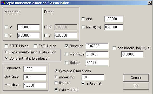
Monomer-Dimer Self-Association Model
Model | Self-Association Models | Monomer-Dimer instant.
Special here are the only the parameters in the upper third, which are those for the monomer and dimer molar masses and sedimentation coefficients. Because the dimer molar mass is twice the monomer molar mass, it cannot be changed.
The field for the dimerization (association) constant will contain the base 10 logarithm of the binding constant in signal units. Assuming, for example absorbance data (with signal a for concentration c), the binding constants in absorbance and molar units would be
![]()
and consequently, the binding constants would transform according to
![]()
(please note that the extinction coefficients should correct for the pathlength 1.2 cm).
If s and D are chosen as parameters instead of s and M (Fit M and s), an analogous box with monomer diffusion coefficient instead of monomer molar mass is used.
New in version 8.7: Hydrodynamic non-ideality has been added to this sedimentation model. The new parameter box for monomer-dimer rapid self-association has an additional check-box to switch ON or OFF (unchecked is OFF, default) concentration-dependent sedimentation, similar to the non-ideal sedimentation model (there's no concentration-dependence of D here). This is for theoretical simulations, fitting of ks can be accomplished in the analogous model in SEDPHAT .
Monomer-Trimer Self-Association Model
Model | Self-Association Models | Monomer-Trimer instant.
Like in the monomer-dimer model, special here are the only the parameters in the upper third, which are those for the monomer and trimer molar masses and sedimentation coefficients. Because the trimer molar mass is three times the monomer molar mass, it cannot be changed. The field ctot is the total loading concentration in signal units.
The field for the trimerization (association) constant will contain the base 10 logarithm of the binding constant in signal units. Assuming, for example absorbance data (with signal a for concentration c), the binding constants in absorbance and molar units would be
![]()
and consequently, the binding constants would transform according to
(please note that the extinction coefficients should correct for the pathlength 1.2 cm).
If s and D are chosen as parameters instead of s and M (Fit M and s), an analogous box with monomer diffusion coefficient instead of monomer molar mass is used.
Monomer-Dimer-Tetramer Self-Association Model
Model | Self-Association Models | Monomer-Dimer-Tetramer instant.
Like the previous self-association models, special here are the only the parameters in the upper third, which are those for the monomer and oligomer molar masses and sedimentation coefficients. Because the oligomer molar masses are calculated as the integral multiples of the monomer molar mass, it cannot be changed. The field ctot is the total loading concentration in signal units.
The field for the dimerization (K12) and tetramerization (K14) association constant will contain the base 10 logarithm of the binding constant in signal units. Transformation from molar to signal association constants works similar as in the monomer-dimer and monomer-trimer model. (The optical pathlength 1.2 cm should be considered.)
If s and D are chosen as parameters instead of s and M (Fit M and s), switching to the monomer-dimer-tetramer model will automatically change the parameters to s and M.
Monomer-Tetramer-Octamer Self-Association Model
Model | Self-Association Models | Monomer-Tetramer-Octamer instant.
Like the previous self-association models, special here are the only the parameters in the upper third, which are those for the monomer and oligomer molar masses and sedimentation coefficients. Because the oligomer molar masses are calculated as the integral multiples of the monomer molar mass, it cannot be changed. The field ctot is the total loading concentration in signal units.
The field for the tetramerization (K12) and octamerization (K14) association constant will contain the base 10 logarithm of the binding constant in signal units. Transformation from molar to signal association constants works similar as in the monomer-dimer and monomer-trimer model. (The optical pathlength 1.2 cm should be considered.)
If s and D are chosen as parameters instead of s and M (Fit M and s), switching to the monomer-dimer-tetramer model will automatically change the parameters to s and M.