In SedPHaT, you can start the non-linear regression for a single experiment or for all of them. Limiting the regression can sometimes be useful at a first stage in order to converge parameters for which a particular data set has very significant information without swamping it with the data from all other experiments. It can also be useful to converge the local parameters (such as local concentrations), before doing a global fit, to avoid poor initial estimates of local parameters throw off the global parameters.
You can interrupt a fit by pressing any key. This will execute the model for the so far best parameters found. (Don't press a key twice in a short interval, in order not to abort the calculation of the so far best model.)
If you have specified a configuration filename, then a new set of "*.sedphat" files and "*.sedphat_PAR" files (and copies of the xp-files) will be generated that stores the so far best intermediate results during the optimization (the names will be preceded by '~'). This enables the restoration of the so far best fit in case the optimization crashes lateron or is lost for some reason.
![]()
There are three fitting algorithms: Marquardt-Levenberg, Nelder-Mead simplex, and simulated annealing.
You can switch between them using the Options->Fitting Options functions. They behave differently. If all algorithms converge to the same solution, then this is likely the overall best-fit (for fundamental reasons, there's no such thing as a guarantee in non-linear regression).
For a description of what exactly is being optimized, i.e. what the goodness-of-fit criterion is, see the statistics page.
Marquardt-Levenberg is based on numerical derivatives of the error surface, which makes it usually fast. It is typically also very good for final convergence, i.e. to home in a fit that is already close to a minimum. It is also good in complicated error surfaces. However, it is susceptible to being trapped by local minima.
Because of the property to home-in well to the minimum close-by, this method can be the method of choice in conjunction with Monte-Carlo error analysis.
Nelder-Mead simplex optimization
is based on geometrically generating a series of down-hill points in the error surface. It starts out with seed points randomly generated around the starting values. It's usually more stable but a bit slower than Marquardt-Levenberg. Disadvantage of Nelder-Mead is that it sometimes can go in circles around a minimum and get stuck. An advantage is that it can be more tolerant of local minima.
I like using both Nelder-Mead and Marquardt-Levenberg sequentially. If you're caught in a local minimum, the random initialization of the Nelder-Mead can help you jump out and get free. Likewise, you can make sure that the Nelder-Mead doesn't merely circle the minimum by executing the Marquardt-Levenberg.
This method is particularly well-suited to explore complex error surfaces with many local minima. In practice, for example, sedimentation equilibrium models of interacting systems may benefit from this algorithm.
The basic idea of simulated annealing is to start out with an ensemble of randomly chosen points (initialized around the starting guesses). Much like in the Nelder-Mead simplex, trials are made to test if each point can be improved by moving it to a different position. Different from Nelder-Mead, however, points will be accepted even if they are actually worse than the original points, but not more than a certain 'temperature factor'. This allows the points to spread in the parameter space. Since this procedure will not lead to convergence, after a fixed number of optimization steps, the temperature factor will be lowered. This will be done in several rounds of lower and lower temperature (annealing), until the temperature factor is 0 - meaning strict optimization.
Input is required for the following:
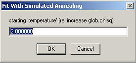
The initial temperature factor (this is simply the tolerated relative increase of the global chi-square). Next, the number of temperatures used needs to be specified
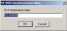
The temperatures will be spaced logarithmically decreasing in the specified number of steps.
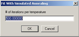
The number of iterations per temperature are the number of simplex steps executed until the temperature is lowered.
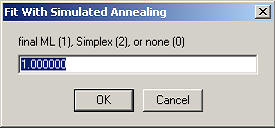
Finally, it can be specified if automatically a final Marquardt-Levenberg step shall be executed (to home in no the minimum), or another simplex at zero temperature.
The implementation used is a combination of Nelder-Mead simplex with simulated annealing as described in Press et al. Numerical Recipes in C.