The measure for the goodness of fit used in SEDPHAT is the "reduced chi-square", calculated as
where the index 'e' refers to the individual experiments loaded, which have N(sub e) data points a modeled with the fit values f. The data points in each experiment have an experimental error sigma(sub e), which is assumed to be Gaussian and uniform within each experiment. The sigmas can be adjusted for each experiment in the experimental parameter box (the noise field). If the sigma values (the noise field) are properly adjusted to represent the true experimental noise of the particular experiment, this reduced chi-square should have a value of 1 for a perfect fit, and all data points from all different experiments are weighted equally in the global fit.
(We could make sure we have the correct sigma values by doing a non-parametric or vastly overparameterized fit, and take the rmsd of a virtually perfect fit as an estimate of the error of data acquisition; however, consider the following...)
However, this usually not the case, since it makes a lot of sense to give different experiments different weights. This is because different experiments differ substantially in their numbers of data points and the susceptibility to systematic errors, and to ignore this could mean to vastly overemphasize the information content of experiments with many data points. If the true standard deviation of data acquisition is indicated as a sigma*, and if we introduce a statistical weight w(sub e) for each experiment, we can rewrite above reduced chi-square as
From this, it can be seen that we can utilize the entry in the noise field to represent the true sigma of data acquisition divided by the weight w, then we will overemphasize the experiment with the factor w^2.
A practical example: The default noise setting for sedimentation velocity is 0.01 signal units, but for sedimentation equilibrium it is 0.005 signal units. This reflects in part that really the noise of an equilibrium experiment is usually smaller, because longer data acquisition can be used (higher 'number of averages in the centrifuge software settings'). However, if we want to perform a global fit of velocity and equilibrium data, consider the following: The velocity data will typically have 100-fold more data points. This would tend to give the velocity data much more weight, and a tiny relative improvement of the velocity fit may swamp a poor fit of the equilibrium data. However, the velocity data are more susceptible to imperfections, for example from convection, and we are perhaps more willing to have a slightly less stringent criterion for the goodness of fit than for the equilibrium experiment. To make the equilibrium experiment count the same as the velocity experiment, we may want to make up perhaps for the difference in the number of data points. To do that, we could lower the noise field entry by a factor of 10, which would give each equilibrium data point a 100-fold higher weight. This is, of course, a judgment which - for good reasons - may be different for different situations, different labs, and different investigators. As a general guide, I suggest to adjust the different weights such that each experiment contributes information, and no experiment is swamped and rendered irrelevant (than there would be no point in including it in the fit...). The default sigma values in the noise fields in the different experiments attempt to introduce adjustments to this effect, but you probably may have to adjust this when fitting data from different experiment types.
As a side-effect, the numeric value of the 'reduced chi-square' will deviate (for a perfect fit) from 1. In the above example, since 1/100th of the data point is given an extra weight of 100 (by reducing the sigma-value by a factor of 10), the best-fit chi-square value should be approximately 2. This should not worry you, since this leaves both the optimization, and the statistical error analysis invariant, unless we use chi-square statistics directly. The F-statistics is concerned with relative changes in the chi-square values, and therefore independent on the scaling of the absolute value.
Error Analysis
There are three major tools for error analysis:
1) F-statistics
2) covariance matrix
3) Monte-Carlo analysis
In practice, the most reliable approach for error analysis is the projections of the error surface method. Although the absolute value of chi-square (‘global red. chi-square’ in the SedPHaT window display) should not be interpreted without absolute knowledge on the noise in the data, the relative increase of chi-square comparing the original and the new fit is a statistical quantity that can be evaluated using the F-statistics.
For example, to determine the error limits on a binding constant, follow these steps:
0) Make sure you have the best fit. (Repeat the optimization a few times alternating the Simplex and Marquardt-Levenberg method.) Save the current configuration (usually with new xp files).
1) Calculate the critical value for chi-square (Statistics -> Critical chi-square for error surface projections).
2) Set the value of the binding constant at a non-optimal value close to the best-fit parameter (for example, increase log(KA) by 0.1), and fix the binding constant. Keep all other unknown parameters floating just like in the previous fit.
3) Execute a new fit. If the original fit was the best fit, then current fit will have a higher chi-square value. Three things may happen:
3a) If a chi-square value smaller than the original best-fit value is observed, which can sometimes happens with complex error surfaces, you have just found a better fit! Go back to step 0.
3b) If the new value exceeds the critical value, then the modified binding constant is already outside of the error interval. Go back to step 2 and repeat with a smaller step (closer to the previous best-fit.
3c) If the new chi-square value is higher than the original best-fit value, but lower than the critical value, fix log(KA) at a value a bit further from the best-fit value and re-fit. Repeat Step 2/3 until the current chi-square value is exceeding the critical value, indicating that one of the limits of log(KA) error interval has been found.
4) Reload the best-fit configuration and repeat the procedure 2/3 by changing log(KA) in the other direction.
is explained in detail in the SedfiT help section on F-statistics. It is based on generating a series of fits, constraining the parameter in question to non-optimal values (starting close to the optimum and moving away), and observing at which point the resulting fit (optimizing all other parameters) worsens the chi-square by a certain critical factor. The implementation of this is straightforward in SedPHaT. The critical values of the reduced chi-square are calculated in the function "Critical chi-square for error surface projections". The approximation used is that both numbers of degrees of freedom are equal to the number of data points. This is a very good approximation for global fits with lots of data points. (A more exact value can be calculated using the calculator in SedfiT after counting the number of fitted parameters.) For details, see Bevington: Data Reduction in the Physical Sciences.
is based on the local approximation of the error surface as a paraboloid, which permits for linear models the exact prediction of error intervals. It is quite fast, but because it is based on a linearized approximation of the error surface in the minimum, it usually significantly underestimates the real errors associated with the parmeters. (In the implementation in SedPHaT, it uses numerical differentiation like the Marquardt-Levenberg algorithm [Press et al.])
Note: Although the error estimates from the covariance matrix are not always realistic, the covariance matrix is an excellent tool to study parameter correlation, and to compare error estimates under different configurations of floating parameters. For example, in some cases the consideration of radial-dependent systematic noise for multi-speed sedimentation equilibrium data can significantly increase the uncertainty of the parameters. This will be reflected in the covariance matrix calculated with and without the TI noise. If, after switching the TI noise on, the covariance matrix does not change much, then the TI noise is well-defined by the data and does not correlate with any of the model parameters of interest.
An example of the output of the covariance matrix looks like this:

In the first line, you find the chisquare of the fit. The second line is the best-fit parameters (this is useful in order to figure out the sequence of how the global and local parameters are listed). The third line is are the normalized gradients of the error surface. Then comes the covariance matrix. The most important numbers are in the second column and are given in parenthesis: these are the error estimates associated with the parameters on the left.
is in theory a very safe way to calculate errors: It is based on generating hypothetical data sets based on the best-fit distributions but with a new set of normally distributed noise (this is the way it's implemented in SedPHaT). Each set is analyzed, and from many hundred or thousand of iterations a distribution of the parameters is calculated, which contain the uncertainties for each parameter. (See also the Monte-Carlo analysis for distributions in SedfiT).
In practice, the drawback of the Monte-Carlo method is that it may not be easy to really optimize each generated data set. In particular with complicated error surfaces that have flat minima, I have observed incorrect optimization causing errors in the parameter distributions. This is due to a fundamental problem that no optimization algorithm can guarantee that the global minimum has been found. I would recommend the Monte-Carlo for cases when you can easily converge with the Marquardt-Levenberg algorithm to the global best-fit. In complicated cases of global fits where you need to switch back and forth from Marquardt-Levenberg and Nelder-Mead to find the optimum fit, I would advise against the Monte-Carlo analysis and recommend the F-statistics instead. (In F-statistics, you have control at each stage to make sure you are really optimizing the parameters.)
For executing the Monte-Carlo analysis, you need to specify the number of iterations (test things out with 100, first, and then go to 1000 or more), the confidence level (default is 0.68), and the directory where to put the intermediate results. If you already did part of the Monte-Carlo in the identical configuration, you can add the new iterations to the previous ones. You will see the progress for each iteration in the SedPHaT window. In the end, you will get output of the following form:
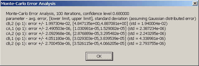
Each row corresponds to one parameter. First is the parameter name, then the average bi-directional error (averaged between plus and minus direction), then the parameter interval comprising the central percentile (i.e. central 68% of the data for 1 standard deviation), and, for comparison, the simple standard deviation assuming that the parameter values are distributed normally.
The regularization menu is for continuous distributions in SedPHaT, which are not yet released for the most part. You'll be able to switch here between different regularization procedures (see regularization in SedfiT).