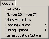

This is where you can set the global partial-specific under standard conditions. For details, see the Partial-specific volume page of the Concepts.
![]()
Under suitable conditions of two or more experiments with sufficiently different solvent density, it is possible to treat the partial-specific volume as a fitting parameter. For details, see the Partial-specific volume page of the Concepts.
![]()
The mass action law calculator will use the currently selected model, ask for total concentrations of A, B, and/or C (dependent on the model), and will report the partial concentrations of all species.
![]()
![]()
Two loading options are available that permit
1) ignoring spikes in sedimentation data; for details see the corresponding SedfiT help website. To utilize features that are available in SedfiT but not in Sedphat, load the data in SedfiT and use the 'Save Raw Data' command to save the preprocessed experimental data into a new directory. Load those in Sedphat.
2) utilizing the combined elapsed seconds and the w2t entry of the centrifuge files to calculate the rotor acceleration. Rotor acceleration will built into the Lamm equation solutions. See the corresponding SedfiT help website.
Both are by default switched on.
![]()

SedPHaT has two fitting options:
1) Fit M and s
This switches the non-interacting species model from (M,s) as free parameters to (D,s). Either way, the Svedberg equation predicts the third parameter of the triple (M,D,s). For details, see the corresponding function in SedfiT.
This switches from Marquardt-Levenberg to Nealder-Mead simplex optimization. Note that the different algorithms can perform differently for different tasks. If you're not familiar with them, I recommend using them both to make sure that a global minimum has been attained. See the Fit section.
![]()

general settings:
1) Set s for changing methods: By default, Lamm equations are solved with the moving frame of reference finite element method for s-value higher than a threshold. Default value if 5. Dependent on the specific problem, infrequently, this value may have to be changed to ensure optimal performance of the Lamm equation solution. For details, see the corresponding function in SedfiT.
2) Set grid size: This refers to the number of radial increments on which the finite element Lamm equation solver is based. This as a factor determining the precision of the simulation of the sedimentation. The higher the number, the more precise and slower the calculations. A value of 1000 should in most cases give a precision far below experimental errors. Usually, 500 is still an excellent value. In some cases it can be useful to go to lower values. The SedfiT tutorial on solving the Lamm equation gives more information.
3) Maximal relative increase per step: This controls the adaptive time-step for the Lamm equation simulation. Default is the value 1. Smaller values lead to finer discretization in time. If a negative value is entered, it has the meaning of a fixed time-step. For example, -1 will fix the time increments to 1 sec, -5 to 5 sec, etc. (Fixing the time-step is usually not recommended.)
Lamm equation options for sedimentation/reaction systems:
1) maximum relative sedimentation per step: This number controls the adaptive step-size in time of the Lamm equation simulation so that the sedimentation per step across the cell does not exceed a certain value. If the numerical simulation is instable, lower this value. For speeding up the numerical solution, increase this value. A good range is between 0.1 and 1.
2) maximum relative chemical reaction per step: This number controls the adaptive step-size in time of the Lamm equation simulation so that the chemical conversion of species per step across the cell does not exceed a certain value. If the numerical simulation is instable, lower this value. For speeding up the numerical solution, increase this value. A good range is between 0.1 and 1.
3) correction level: This controls the level of refinement of the predictor-corrector scheme. Possible numbers are 1, 2, and 3. Recommended is the level 1. Higher levels produce slightly higher accuracy, but this is usually not significant. Higher levels also are more computationally intensive.
4) fix timestep: This provides the possibility to circumvent part of the the adaptive time-step control, and to fix the time-step to a pre-defined value. For example, enter 1 will make the time-increments uniformly 1 sec. (Default is switched off.)
5) limit stepsize control to fitting limits: The adaptive control of time-steps can optionally be scanning the whole solution column, or only the range between the fitting limits. (Default is the whole range.)
6) shut off back-diffusion: For the analysis of high-speed sedimentation velocity data that does not include back-diffusion from the bottom of the cell, the back-diffusion can also be eliminated from the numerical simulation. This substantially increases the stability and efficiency of the Lamm equation solution. Shutting off the back-diffusion here will eliminate back-diffusion for all experiments loaded. It can also be specified for each experiment separately, in the 'no back-diffusion necessary' field of the sedimentation velocity parameter box.
7) testing mode: allows to specify the molar mass and extinction coefficients of the complexes for each simulation. This can be useful to examine special cases of the Lamm equation solution. (Default is OFF.) Also, setting selectively the extinction coefficient of different species to zero allows to visualize (and copy the data to the clipboard from) the contributions of each species to the fit. --> don't use this setting for fitting; only use it with the Run command.
8) save intermediate results to c:\temp: When this checkbox is checked, for sedimentation velocity simulations of interacting species, the individual concentration distributions of each species in molar units is saved to the harddrive. Only use with the Run command. In conjunction with isotherms using Gilbert-Jenkins theory, the asymptotic boundaries will be saved.