[ sedfit help home ]

[ Up ] [ Load New Files ] [ Set Initial Data ] [ Data Housekeeping ] [ realtime ] [ Export to SEDPHAT ] [ Exit ]

Loading data consists of a few simple steps. It is strongly recommended to read these instructions carefully, as most difficulties in first using Sedfit arise from incorrect loading of data.  According to the principle of direct boundary modeling, there is no need for any data transformation, alignment, or any other operation.  (Systematic noise will be calculated algebraically, see systematic noise analysis.)  

Some information on experimental conditions is given in the tutorial on size-distribution analysis.  Also, considerations for setting the meniscus and the fitting limits are described in the tutorial. 

1) Opening the data files

When loading data, the dialog box for selecting a number of data files appears. Selection follows the usual Windows conventions (i.e. navigation to the directory, selection of filters, marking files either by holding ctrl-key and click on each file, or (better) by holding the shift key and clicking on the first and last)

!    (in a real example, for direct boundary modeling it is always recommended to analyze as large a data set as possible, which usually is the entire available data. Exceptions are the van Holde-Weischet procedures for diagnostic purpose)

New in version 9.2:  Drag-and-drop loading of files into SEDFIT is possible.  This substitutes the use of the menu function Data->Load New Files and the use of the file selection box.  Everything else that follows is the same.

This is straightforward, but there are a few rules: 

* make sure that by use of the appropriate filters, e.g. by typing *.ip1, only scans from a single cell are loaded (New: Please note the new preset file filters in the "files of type" menu.)

* it is not necessary to select by hand 'every n-th file', as this can be selected later in a box that will pop up:

entering 1 will load all files, 2 every second, 10 every tenth, etc. This can allow to speed up a first rough analysis of interference data.

* permission to write to the drive containing the data is required.  This means that data cannot directly loaded from a CD, or certain network drives (in this case, the data should be temporarily copied to a drive with write permission, such as a local hard drive).  The reason is that several new files will be written into the data directory.

* more than one file has to be loaded

!    instead of a selection of multiple files, a file 'list.ip1' (or analogous) previously generated by SEDFIT can be selected.  This file contains all information about the complete previous set of files, and can be edited by a text-editor such as notepad.  (After moving the data to a different location,  the first line in the list-file may have to be edited to reflect the correct new pathname.  Further editing can be done by inserting a '%' at the beginning of a line with a particular filename, this will omit the following file from being loaded) 

* if files are loaded from a previously analyzed experiment, a box appears

'yes' will restore the previous analysis, including meniscus and bottom setting. Currently, this will work for c(s), c(s,f), c(s) with discrete component, and c(s,f) with discrete component models.

!    the parameters from a previous fit are stored in a file '~tmppars.ip1' (or analogous).  This file can be inspected and edited with a text editor (see format of the ~tmppars file).  When the program previously crashed during the fit, the best fit up to the time of the crash will be reloaded (see FAQs)

* there are a large number of loading options, including elimination of spikes, filename convention, file formats, handling of rotor acceleration, data transformations, etc.  Some of these can have an influence on the numerical details of the data loaded. Another function allows to multiply the data by -1, in case the sample and reference side of the centrifuge cell have been inadvertently switched. 

* there will be an automatic check if the temperature was stable during the run.  If there was a drift by more than 1 degree, the temperature plot a warning message will appear.  

2) Inspecting the data plot and setting meniscus and bottom 

After successful reading of the data files, the SEDFIT window will show two plots, the upper one for the data and fit, the lower one the residuals.  The appearance of these plots can be changed in the display menu and additional information (data filenames, residuals bitmap, etc. can be retrieved).  

However, initially there's no fit and therefore the residuals plot shows the entire data (unless a previous fit is being restored):

Note the red and the blue lines in the upper plot.  They denote meniscus and bottom of the solution column, respectively.  By default, after loading the data, they are just set to the innermost and outermost radius of the data.  Because Lamm equation analysis requires knowledge of the boundaries of the solution column, the meniscus and bottom must be set by the user.  

!    later on, the meniscus and bottom position can also be entered numerically, and be refined by nonlinear regression (see fit parameters).

!    if a previous analysis has been performed already after starting SEDFIT, the window will already have meniscus and bottom positions, as well as green lines indicating the radial range for fitting.  These values can be accepted, if they represent good values for the new data, or new positions can be entered, ignoring the old location.  Sometimes, if the previous data span a completely different range than the new data, the meniscus and bottom may be out of range of the data plot.  In this case, it can be easier to enter the meniscus and bottom numerically (see fit parameters) 

Graphically entering the meniscus is done the following way:  

a) hold the control-button pressed, and left-double click with the mouse at the radial position where the meniscus likely is located.  This will generate a black line, and the radius value of the location will be printed. 

!    if not satisfied with the position of the black line, it can be re-entered in the same way (by ctrl-left-double-click), or by shifting it with the arrow keys.  For better inspection of the data, the view can be changed, e.g. spanning a view rectangle with the right mouse button, as described in the display menu.  If the process of graphical entry of a data limit shall be aborted, press the Esc key.

To confirm the current position, press the Enter-key (or the tab key). This will make a new red line at the new meniscus position. Note that the old red line, for economic reasons, will not immediately erased, but only after the windows is redrawn. (This can be forced using the display update menu function.)

Please note that the graphical determination of the meniscus position should always be done with the raw data! (Systematic noise subtraction can obscure the meniscus artifacts.)

b) we set the bottom position in the same way:  ctrl-left-double-click to the position where the bottom is located.  This will also generate a black line at the new position (here at 7.2 cm).  

If satisfied, we confirm the position with the Enter key or the tab key. This will set the new bottom position, and a new blue line will appear:

you can ignore the old red and blue lines, or else force a redraw of the screen.

!    SEDFIT distinguishes meniscus and bottom because of their relative position, and it interprets any new limit as a relocation of the solution boundary it is closest to.  This is very convenient and works well in most cases.  Sometimes, however, when the data span a much larger radial range than the actual solution column, some confusion between meniscus and bottom can appear.  In this case, it can be necessary to set the meniscus position in several steps.  For example, if the data were recorded from 5.8 cm to 7.2 cm, but the actual solution is only from 6.9 cm to 7.2 cm, then entering a limit at 6.9 cm will be interpreted wrongly as a new bottom location.  This can be avoided by setting first an intermediate meniscus position to 6.2 cm, then to 6.5 cm, 6.8 cm, and finally to 6.9 cm.  This sequence does not move the meniscus more than 50% of the distance meniscus - bottom in any single step, and therefore SEDFIT does not get confused.   

Note in version 11.0 (December 2007) and later: All limits can now be moved around by dragging with the mouse

3) Setting the data range suitable for analysis

Because not all the data between meniscus and bottom can be analyzed, due to the unavoidable optical artifacts close to the solution boundaries, we have to set the inner and outer data analysis limit.  This is done very similar to the meniscus and bottom, but without the control-key.  The sequence here is relevant:  First set the outer analysis limit by left-double-click at the maximum radius position that contains artifact-free data.  This will generate a black line: 

If necessary, relocate with the arrow keys, or re-enter it with the mouse left double-click at a new place. Accept the position with the Enter key (or tab key).  This will generate a green line indicating the outer fitting limit:

!    In the Lamm equation analysis procedures of SEDFIT, the back-diffusion from the bottom can be included in the analysis.  In fact, for small molecules this part contains a lot of information.  One should be aware, however, that this makes the bottom position of the solution column an important parameter, and sometimes it is important to optimize the bottom position during the fit (see fit parameters).  If the sample contains only large molecules, however, the back-diffusion regime is very steep and can conveniently be excluded from the analysis.  (If the back-diffusion range is as steep in as in the data shown, for example, the residuals in this range would tend to dominate the overall fit, but not carry a lot of reliable information.)

Note that a second green line has been generated close to the meniscus.  This is only a default position, and in general, next, the inner analysis limit should be set by the user. Left-double-click at the desired radial position.

Here, for example, we have moved the inner analysis limit a little bit further away from the meniscus to make sure there are no meniscus artifacts in the data range for the analysis. Accept the position with the Enter key (or tab key). 

!    The data range in between the green lines must be common to all data sets.  If there's a data set that does not span the same data range, an error message will be generated (see FAQs), and the green lines will be adjusted to the maximal possible range. 

At this point, I recommend to force a screen redraw, for example by using the Display->Update command.

Please note that we have now have (from left to right) a red line at the meniscus, followed by a green line indicating from where we trust the data being artifact free, followed by another green line indicating the end of our fitting range, and finally a blue line indicating the bottom position. The residuals plot (lower plot) now only shows data in between of the green lines, i.e. in the data analysis range.  

That's all that is required for loading data.  More data files of the same experiment can be loaded by using the function Add More Files. 

Note in version 11.0 (December 2007) and later: All limits can now be moved around by dragging with the mouse

Further, the different filenames associated with the scans appear when moving the mouse across the scan or residual, here, for example, scan #34.

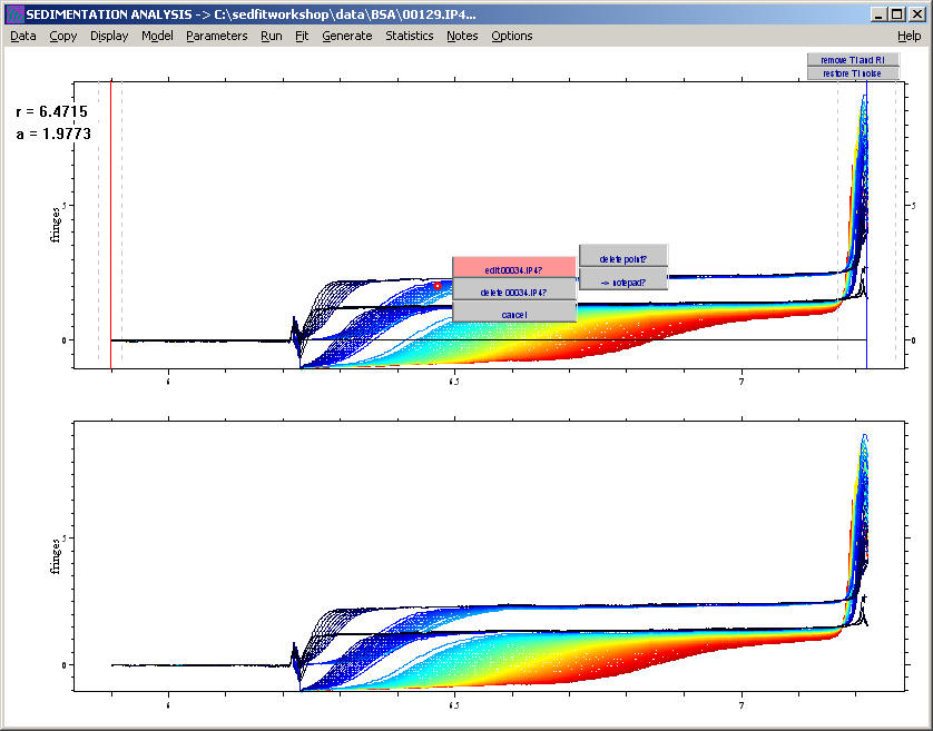
clicking the left mouse button then makes a menu appear with clickable buttons

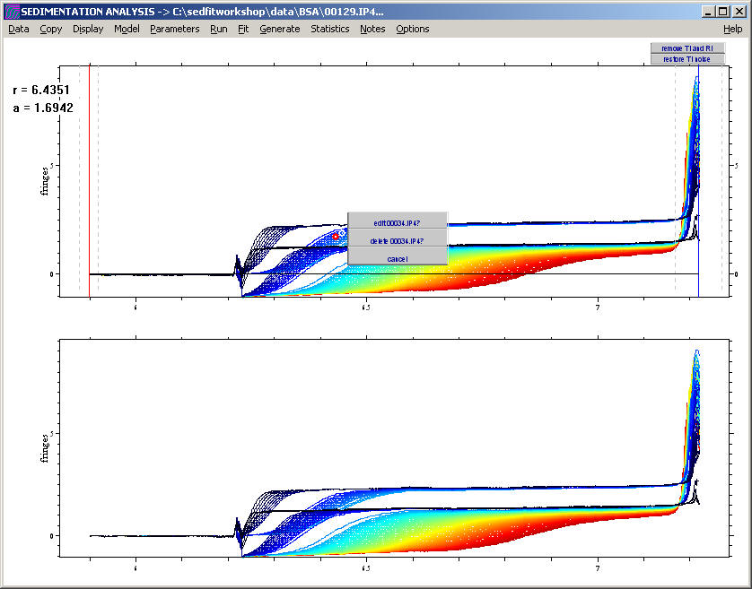
The "edit" button allows to either edit the scan in the notepad, or simply delete a single data point.

Variants:  Sedfit can also work with data from dynamic light scattering, and  XLA/XLI sedimentation equilibrium data files.

1) Loading DLS data: For DLS data, first several raw autocorrelation data sets from Protein Solutions 99 (version 5.20.05), Brookhaven Instruments, or ALV are transformed into a new data format (g(2)-1 as ASCII with header). This is described in generate DLS data file. The generated data format *.dlsdat can then be loaded with Data | Load DLS Data. Of course, the lines for meniscus and bottom become meaningless, but the green lines for the data analysis range keep their function.  The data will be transformed into field autocorrelation functions by using the relationship g(1)² + 1 = g(2). DLS data can be analyzed in terms of size-distribution, diffusion coefficient distribution, or single species (described here), all using the same framework and in analogy to the sedimentation velocity analyses.

2) Sedimentation Equilibrium Data: Equilibrium data can be loaded into Sedfit (Data | Load Sedimentation Equilibrium Data), mainly to allow the use of the size-distribution formalism c(M) for equilibrium analysis.  The c(M) and the independent species model can be used; both will automatically use the appropriate equilibrium model functions.  In contrast to loading of sedimentation velocity data, here only a single file should be loaded. It should be noted that the analysis of molar mass distributions can be very ill-conditioned. When analyzing equilibrium data, concentrations are referring to effective loading concentrations, making use of the specified meniscus and bottom position to integrate through the solution column.

3) Electrophoresis data: Electrophoresis data (with ‘E’ as a type character in the file header) can be loaded in the same way as sedimentation velocity data. The data can be analyzed in analogy to the sedimentation velocity analyses, substituting the s-value by velocities v (in mm/sec), and making use of the fact that the electrophoresis is a process that resembles sedimentation with a constant force and linear geometry. From the velocities and the known field, electrophoretic mobilities can be calculated.  Only the models labeled as electrophoresis analysis can be used.  They are described here. 

This function allows to increase the number of scans that are included into the analysis, by loading additional data files.  This is straightforward, but it should be noted that no provision is made to eliminate duplication of files.  Single files can here be selected.

The additional data files will not be added to the files documented in the file "list.*". If no data previously have been loaded, this will invoke the same function as Data->Load New Files.

This function loads the same selection of scans as currently loaded, but taken from the data of another cell.  This is a convenient way to switch to the analysis of similar data in the other cell.