Independent Species Model
Model | Non-Interacting Discrete Species
This model describes the concentration distribution of one or more (up to four) non-interacting and ideally sedimenting species. In case of more than one species, the model functions are superpositions of the distributions of the individual species. The concentrations of each species are expressed in the total loading concentration and fractional loading concentrations.
If the number of species is not well known (including knowledge of possible small fragments or larger aggregates), it can be determined in a c(s) analysis as the number of peaks in the continuous sedimentation coefficient distribution. From this analysis, also the starting values for the s-values of each species can be taken. This is illustrated in the example of how to use Sedfit.
This model allows to calculate the concentrations, molar masses, diffusion coefficients, and the sedimentation coefficients of discrete species. Starting guesses for s and M (or D) must be provided, and can be optimized by non-linear regression in the fit command. Because this model is linear in the concentration of each species, no starting guesses for the concentrations are necessary - they will be optimized already with a simple run command.
For non-interacting ideally sedimenting molecules, sedimentation is described by the Lamm equation
![]()
It describes the evolution of the concentration ck(r,t) of a species with sedimentation coefficient s and diffusion coefficient D in a sector-shaped cell, and in the presence of a centrifugal field with angular velocity w). In Sedfit, the Lamm equation is solved numerically by the finite element technique. Details on the solution of the Lamm equation are described here (and in refs 1 and 2). Although the primary measured parameters in a sedimentation experiment are s and D, the parameters can be transformed to s and M by use of the Svedberg equation
![]()
(see Fit M and s). In this case, the partial-specific volume and solution density has to be specified (see set v-bar and rho). Using M as the boundary spreading parameter can allow input of the frequently known molar mass, or simpler interpretation of oligomeric stoichiometry, and this setting is therefore the default. On the other hand, the diffusion coefficients may be known from dynamic light scattering experiments.
A number of variants are available, as well as fitting options.
The parameters for this model are entered in the parameter input box (Parameters):
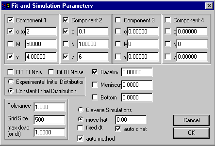
upper section specifying
up to 4 components
middle section with experimental conditions
lower section with Lamm equation and
nonlinear regression parameters
Note: for a generalization of this model, look at the SedPHaT hybrid continuous/discrete model.
The upper sections specifies the parameters for each of the four components (or species), each with four controls:
1) The different components are switched on/off according to the status of the check-mark next to the label 'component 1', 'component 2', etc. If the species are switched off, it's sedimentation will not be simulated and it will be ignored. (It should be made sure that no parameters of this component are marked for non-linear optimization). In the parameter box shown, for example, only 2 species are used.
2) the concentration field gives either the total loading concentration (for the first active component), or a fraction of the total loading concentration (all following concentrations). In the example above, the total concentration is 2, and the concentrations of species 2 is 10%, which means the concentration of species 1 is 1.8, that of species 2 is 0.2. The units are signal units, i.e. interference fringes or OD1.2 cm at the wavelength chosen. If the check-mark is switched on, then the concentration will be optimized. Because the loading concentrations are linear parameters in this model, if checked, they will be optimized in both the run and fit commands.
3) the molar mass or diffusion coefficient field contains the information governing boundary spreading. If the parameters are set to (s,M) the field is labeled 'M' (as in the example), and entry is the molar mass of the species in units of Dalton. The buoyancy term is governed by the partial-specific volume and buffer density, which needs to be specified here. (Please note that there's only one v-bar for all species, which means the molar mass values may have to be corrected if the different species have different v-bar.) If the parameters are set to (s,D), the field is labeled 'D' and the entries are diffusion coefficients in 10-7cm2/sec (buoyancy parameter are not relevant in this case). This is a nonlinear parameter. If the check-mark is set, this parameter will be optimized in the fit command, while the goodness of the starting guesses can be assessed (no optimization) with the run command. The parameter may also be constrained to the value shown (check-mark absent), which can be useful, for example, if the molar mass of the species is known.
4) the sedimentation coefficient field shows the s-value of the component in Svedberg units. Because this is a nonlinear parameter, it will be optimized only if the check-mark is set and the fit command is used. (For flotation, use negative values and set v-bar = 0)
The middle section contains controls that depend on experimental parameters. The parameters of the middle and lower section are parameters common to many models. These are:
1) a checkbox ‘FIT TI Noise’. If checked, the boundary analysis is combined with an unknown radial-dependent background profile that remains constant in time (Time Invariant). This is calculated algebraically and explicit background profiles are used for direct boundary modeling (see systematic noise analysis, and ref 3). Mostly, this function will be used when analyzing interference optical data, although application to absorbance data can occasionally be useful, too (3). It is switched on for interference data by default. After the time-invariant background is calculated, it can be subtracted from the data for better inspection of the fit. Because this TI noise consists of linear parameters, it will be calculated in both the run and the fit command.
2) a check box ‘FIT RI Noise’. If checked, this adds to the model the possibility of a baseline offset that is constant in radial direction, but different for each scan. Like the TI noise, this is calculated algebraically (see systematic noise analysis and ref 3), each time when the run and the fit command are used. It is switched on for interference data by default, because of the small up-and-down displacement (jitter) always involved in sequences of interference scans. Also, the integral fringe displacement sometimes encountered in interference data can count as RI noise. Please note: No correction for jitter or fringe displacement should be performed before the analysis. The best-fit displacements will be result of the analysis, and can be subtracted from the data after the boundary modeling.
3) the field Baseline allows to enter and optimize a constant baseline that is common to all scans and that is constant in radial direction. If this is checked, it will be optimized with each simulation. It is recommended to keep the baseline parameter floated for absorbance data (except when working with very small molecules and small sedimentation rates, when some correlation with the molar mass can be possible if simultaneously floating the bottom parameter).
4) the Meniscus position of the solution column will generally show the radius value that has been graphically determined when loading the files. However, the value can also be entered or changed here. The value of the meniscus position is very important for measuring the sedimentation velocity. When the field is marked, the meniscus is treated as a nonlinear fitting parameter, to be optimized in the fit command. In this case, constraints for a the lowest and highest possible values are necessary (as judged from graphical inspection of the data), and a prompt will automatically ask for these values when closing the parameter box. They should be carefully entered, since the default interval could be off. The range constraints can also be set through the fitting options.
5) the Bottom position of the cell is shown here, as graphically entered. Analogous to the meniscus field, it can be entered or modified here. Also, the bottom value can be treated as a fitting parameter (when checked) to be optimized in the fit command. Also, constraints for a the lowest and highest possible values are necessary when floated, and a prompt will automatically ask for these values (which can be modified through the fitting options). Fitting for the bottom position is very important when back-diffusion of the species from the bottom is modeled, because the exact bottom position is very difficult to locate graphically. Analysis with floating bottom will mostly be required for small molecules with high diffusion constants, at low rotor speeds, or in approach-to-equilibrium analyses. It should be noted, though, that in approach-to-equilibrium analyses at low rotor speed the simultaneous floating of the three parameters bottom, baseline, and molar mass can lead to slight correlation (although generally any two will be well-determined).
A number of variants of the non-interacting models are available, including those with modified initial distribution (for analytical zone centrifugation), and different geometries (linear Lamm equation and electrophoresis). Further, it is possible to include the starting time of sedimentation as a fitting parameter (this is for empirical fitting of the approach to equilibrium), or treat the sedimentation coefficients as a time-dependent quantities and analyze s(t).
Please note: Starting from version 8.5, when using this model with s and D as fitting parameters, there will be the option to consider (and fit for) non-ideality parameters for the first component.