
Note from version 4.0 and up: The appearance of the parameter input boxes for interacting systems will depend on the data type loaded. The goal is to simplify the parameter entry by eliminating irrelevant parameters . For example, enthalpy number are only required in ITC experiments, and kinetic rate constants currently only for sedimentation velocity.
NEW version 2.0: All hetero-association models for sedimentation velocity can incorporate both slow and fast reaction kinetics.
This is in addition, to the previous implementation for sedimentation equilibrium experiments (single and multi-speed) and for isotherms.
Points to keep in mind:
* concentrations are in micromolar units, utilizing the extinction coefficient A and B values from the Experimental Parameters box.
* association constants are directly in log10 of molar units (for example, for a value of log10(Kab) = 5 means KD = 10 mM)
* local parameter menu will be the effective loading concentration for each experiment in micromolar units.
* incompetent fractions can be considered for component A and for B
* component B can be specified in molar concentration or in molar ratio
* a species not participating in the association can be specified (check the 'add non-participating species' field) This is simply an additional component, perhaps an impurity, which has nothing to do with the associating molecules.
Note: because there is only input of a single partial-specific volume, the molar mass values will have to be adjusted accordingly to produce the correct buoyant molar mass. This is outlined in detail in the Partial-specific volume page of the concepts.
All models provide the possibility of adding an additional species that is unrelated to the reactive species.
This can be used to describe, for example, a contaminant, or IF signals from sedimenting buffer salts. The presence of such components, and their estimated molar mass and s-value may be obtained from c(s) analysis with sedfit. The purpose of the vbar in this section allows this species to be used in a flexible way in density contrast experiments (e.g. to describe the free detergent micelle).
Currently (version 1.5) there are only 2 models: A + B <-> AB for the reversible association of two components which don't self-associate and have a single site, and a two-site model A + B + B <-> AB + B <-> ABB.
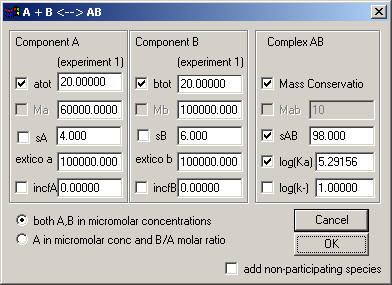
There are separate fields for component A and B. If you check atot (or btot, respectively), the loading concentrations of A will be floated in the analysis. You need to determine the molar mass of A and B separately. The extinction coefficient is shown here (taken from the first experiment), but it will have to be entered in the Experimental Parameters box. The fileds 'incfA' and 'incfB' are for the fraction of incompetent A and B.
On the right, you can switch on mass conservation (if fulfilled) for the sedimentation equilibrium analysis. (I suggest to use this in multi-speed long-column sedimentation equilibrium experiments in conjunction with floating bottom positions.).
On the right is also the entry association constant; note that the default value for log10(Ka) is at 1, essentially switching off any interaction.
Obviously, the log(k-) entry only gains meaning for the sedimentation velocity models. The log(k-) is the base-10 log of the chemical off-rate constant of the complex. Values of > -1 (k- is faster than 0.1/sec) will switch the simulation to instantaneous equilibrium with mass action law fulfilled at all times and positions throughout the cell. Values smaller than -6 (koff < 1x10(-6)/sec) will lead to sedimentation profiles nearly identical to those of independently sedimenting populations of the free and complex species of the loading mixture.
Below, you can switch to either have both A and B specified in micromolar concentrations (this will be done in the local parameters menu), or A in micromolar units combined with B being the molar ratio B/A. Dependent on how the experiment is setup, you may have different cells with the same molar ratio, hence in the global analysis you might be able to share molar ratio parameters. Alternatively, if you have in different cells component A at a constant concentration, you will be able to share the loading concentration of A among these cells.
Everything else is the same as usual.
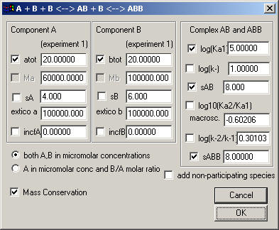
This is a good model for a component A which as two equivalent (or two different) sites for a component B. There can be cooperativity between the sites.
This is pretty much like the model before, except that there are two association constants: Ka1 for the binding of a first molecule B to A, and then Ka2 for the addition of a second B to the pre-existing AB complex. Instead of using two separate association constants, the model is expressed here in terms of a macroscopic association constant Ka1 for the first binding, and the ratio Ka2/Ka1 for the second.
Likewise, the off-rate constant of the ABB complex is expressed as the base-10 log of the ratio of the off-rate constant of first and second complex. Obviously, the log(k-) entry only gains meaning for the sedimentation velocity models. If both off-rate constants are > 0.1/sec, this will switch the simulation to instantaneous equilibrium with mass action law fulfilled at all times and positions throughout the cell. Values smaller than -6 (koff < 1x10(-6)/sec) will lead to sedimentation profiles nearly identical to those of independently sedimenting populations of the free and complex species of the loading mixture.
Otherwise, the model works very similar as all the others.
For equivalent sites with no cooperativity, the log10 of this factor Ka2/Ka1 is -0.602. This is because of the statistical factors, which for equal microscopic constants produces a factor 1/4 for the macroscopic constants. Any deviation from this means that there is cooperativity between the equivalent sites. For the stability of the complexes, equivalent sites will lead to a factor 2 for the koff(ABB) versus koff(AB), because of the two possibilities to dissociate one of the ligands.
In this way, you can make the analysis with the constraint that the sites are equivalent (by fixing the log10(Ka2/Ka1) to the default -0.602, and by fixing the log(k-2/k-1 to 0.301).
Note: Because Ka1 is the macroscopic constant and A has two equivalent sites, the Ka1 is a factor of 2 larger than the microscopic Ka of the simple A+B<->AB model. Therefore, to get to the microscopic binding constant divide Ka1 by 2, and to get to the microscopic cooperativity, multiply Ka2/Ka1 with a factor 4.
Examples for equivalent sites are antibodies binding up to two antigen molecules, or a receptor dimer binding one or two ligand molecules.
For non-equivalent sites with no cooperativity, we determine the macroscopic constants Ka1 and Ka2 (Ka2 = Ka1*10^(log10(Ka2/Ka1)). The microscopic constants Kmic1 and Kmic2 are given by Ka1 = Kmic1 + Kmic2 and Ka2 = Kmic1*Kmic2/(Kmic1 + Kmic2). This will lead to macroscopic constants that are at least a factor 4 apart, i.e. our parameter log10(Ka2/Ka1) must be smaller than -0.602. This leads to Kmic1 = (1/2)*(Ka1*{1-sqrt[(Ka1-4*Ka2)/Ka1]}, and Kmic2 = (1/2)*(Ka1*{1+sqrt[(Ka1-4*Ka2)/Ka1]}.
Examples for distinguishable sites are proteins that just have to happen to different binding sites for the same ligand, but the sites are at different places of the same protein and have different types of binding interfaces for the ligand.
For non-equivalent sites with cooperativity, the situation is more difficult and one will not be able to determine the binding site heterogeneity and microscopic cooperativity. Please consult Enrico DiCera's book "Thermodynamic Theory of Site-Specific Binding Processes in Biological Macromolecules", chapter 3.