This model fits all active data globally with up to 4 independent species. The specific characteristics of this model is that no assumption on the population of the different species, their signal increment, and relationship between different experiments is made. All data sets are simply fit by a combination of these species, without regard for the signal amplitudes of the contributions of each species. However, all experiments are fit with the same M, s, D values for each species. The basic question is here - 'what's in there' and not 'how much'.
There are no local parameters to set, because all partial concentrations are linear fitting parameters. Also, there are no shared concentration parameters. Partial concentrations for each species (and each data file for multi-speed equilibrium experiments) are given in the text output on the screen, in signal units. For sedimentation equilibrium, the reference radius is the bottom position of the cell.
It does not make sense in this model to float meniscus or bottom position of sedimentation equilibrium experiments. There's no mass conservation for sedimentation equilibrium (that's in a different model, see here).
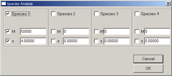
This is the parameter box:
The parameter box works similar as the one in SedfiT. In the upper half, it has 4 fields, one for each species. You can activate a species (include it in the fit) by checking the box in the upper left corner of the field. Specify the molar mass and s-value accordingly, and check the values if you want to optimize them in non-linear regression. Everything else has pretty much the same meaning as in SedfiT.
Note that you can select the Marquardt-Levenberg optimization algorithm, the default is simplex algorithm.
Each value of M and s automatically determines D via Svedberg equation. You can switch to a basis of s and D using the 'Fit M and s' toggle in the options menu.
If you need more species, use the hybrid local continuous and global discrete model, which has up to 10 species.
Please note: Do not enter s-values of zero, these components will be switched off, even in sedimentation equilibrium. When dealing with sedimentation equilibrium experiments only, do not optimize s-values.
This model is for sedimentation velocity only. It is a way to extract very simple information from the translation and diffusional spread of the sedimentation boundary, based on the Faxen approximation of the Lamm equation.
The application of this model requires data that are free of systematic noise parameters. This can be achieved best by fitting the data with a continuous c(s) model (making sure it is an excellent fit),and using the function "Data -> Copy all data and save as new config" and agreeing to the option to subtract TI and RI noise from the data". This step is necessary because only a certain user-defined percentile of the boundary will be fitted, and this requires the assessment of the boundary height for each scan. In the new xp-file, uncheck the TI and RI noise box. Then switch to the Linear Fractional Boundary Model. The parameter box looks like this:

Mapp is the molar mass derived from the slope of the boundary, and s the s-value from the translation. The "boundary fraction fitted" determines the size of the central portion of the boundary to be fitted. For example, 0.8 means the boundary will be fitted between 10% and 90% of its plateau value. 0.5 would mean the fit will take from 25% to 75% of the boundary, which is used in the following example:
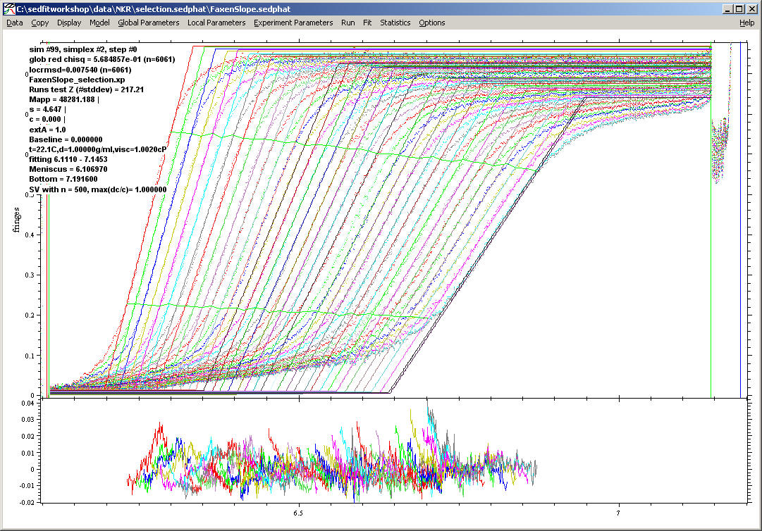
As can be seen, the fitting function is only a diagonal line, which is aimed at fitting the central slope of the boundaries. The fitted data are indicated by the horizonal green lines, which indicate the lower and upper limit of the data.
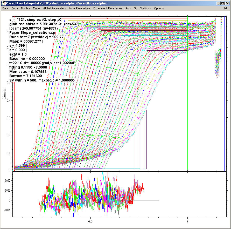
Note: To establish the plateau level, the conventional radial fitting limits (indicated by the vertical green lines) must be at least 0.1 cm from the boundary (i.e. at least 0.1 cm plateau must be established) in each scan to be included in the fitting. Below is a setting where this conditions is not fulfilled. Notice the step-functions in the fitted distributions, which indicate the absence of a suitable plateau. They will not be included in the fitted data.
Obviously, this is not a precise way to determine the molar mass. Many other models will be much better for that. However, the linear boundary fraction model can serve as an empirical parameterization of the boundary. This can be useful for 'model-free' comparison of boundary shapes, for example, where more detailed models are not available.