
These models can be used to globally analyze sedimentation equilibrium and/or sedimentation velocity data.
Note from version 4.0 and up: The appearance of the parameter input boxes for interacting systems will depend on the data type loaded. The goal is to simplify the parameter entry by eliminating irrelevant parameters . For example, enthalpy number are only required in ITC experiments, and kinetic rate constants currently only for sedimentation velocity.
NEW version 2.0: All self-association models for sedimentation velocity can incorporate both slow and fast reaction kinetics. For an introduction to these models, see Sedimentation Velocity for Reactive Systems.
Note: In version 1.5, sedimentation equilibrium models monomer-tetramer-octamer and monomer-m-mer-n-mer are not yet implemented. None of the self-association models is implemented yet for dynamic light scattering.
NOTE: The sedimentation velocity models for rapid reactions are similar to the self-association models in SedfiT, but permit global analysis. There are a couple of important differences:
* concentrations are in micromolar units, utilizing the extinction coefficient A values from the Experimental Parameters box. (The fact that the oligomer has higher extinction is automatically taken care of.)
* association constants are directly in log10 of molar units (for example, for a monomer-dimer association with log10(KA12) = 5 means 1/Ka12 = 10 microM)
* local parameter menu will be the effective loading concentration for each experiment in micromolar units.
* incompetent fractions can be considered
* non-ideal sedimentation can be taken into account
The general properties of these models are described in
P. Schuck (2003) On the analysis of protein self-association by sedimentation velocity analytical ultracentrifugation. Analytical Biochemistry 320:104-124 (preprint)
and a practical example can be found in
S.A. Ali, N. Iwabuchi, T. Matsui, K. Hirota, S. Kidokoro, M. Arai, K. Kuwajima, P. Schuck, F. Arisaka. (2003) Reversible and fast association equilibrium of a molecular chaperone, gp57a, of bacteriophage T4. Biophysical Journal 85:2606-2618
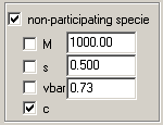
All models provide the possibility of adding an additional species that is unrelated to the reactive species.

This can be used to describe, for example, a contaminant, or IF signals from sedimenting buffer salts. The presence of such components, and their estimated molar mass and s-value may be obtained from c(s) analysis with sedfit.
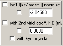
For sedimentation velocity analysis, all models can incorporate hydrodynamic non-ideality (log10[ks/(mg/ml)]) for instantaneous reactions (k- > 0.1/sec).

In sedimentation equilibrium models, only the thermodynamic non-ideality will be used.

The entries of this box are consistent with the conventions of the other parameter boxes.
Note that the log(Ka) is a base-10 log of Ka in molar units. The default starting estimate shown here is Ka = 1x10(5)/M (i.e., monomer concentration = dimer concentration at 10 microM).
Obviously, the log(k-) entry only gains meaning for the sedimentation velocity models. The log(k-) is the base-10 log of the chemical off-rate constant of the dimer. Values of > -1 (k- is faster than 0.1/sec) will switch the simulation to instantaneous equilibrium with mass action law fulfilled at all times and positions throughout the cell. Values smaller than -6 (koff < 1x10(-6)/sec) will lead to sedimentation profiles nearly identical to those of independently sedimenting populations of the free and complex species of the loading mixture.
Tips:
* it is useful to constrain the monomer molar mass, if possible.
* the non-ideality can be switched on (default is off) by checking the box to the left of the 'log10[ks/(mg/ml)] nonid sed field. The non-ideality parameter can be floated in non-linear regression if the check-box next to the number entry field is checked.
* Mass conservation is always implied in sedimentation velocity, but may not always be fulfilled for multi-speed equilibrium experiments. If this is left un-checked (no mass conservation), data sets within one multi-speed sedimentation equilibrium can have different effective loading concentrations.
* the incompetent fraction is 0 by default. To consider the possibility of incompetent protein population, set the fraction value to a number > 0 (and < 1). You can optimize this in non-linear regression by checking the box next to 'fraction'. There are two possibilities: you can have incompetent monomer, or irreversible dimer. For non-participating monomer, enter n = 1 in the corresponding field (default), for irreversible dimer enter n = 2.
The 'Tolerance', 'Gridsize', and 'max dc/c' parameter have the same meaning as in SedfiT.

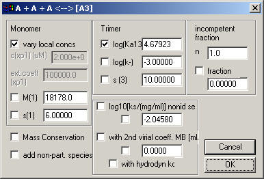
This basically works the same as the monomer-dimer model. Note that the association constant is again the log10 of Ka in molar units. The default starting estimate shown here is Ka = 1x10(5)/M2 , which would correspond to a concentration of equal monomer and trimer at 10-5/2, i.e. 3.1 mM (millimolar). If equal monomer and trimer concentration is at 10microM, that would correspond to a Ka of 1x10(10)/M2. Therefore, if you have micromolar concentrations and some reasonable fractions of the material is trimeric, you should change the starting guess of log10(Ka13) to 10.
The log(k-) entry describes for sedimentation velocity data the stability of the complex. The log(k-) is the base-10 log of the chemical off-rate constant of the trimer. Values of > -1 (k- is faster than 0.1/sec) will switch the simulation to instantaneous equilibrium with mass action law fulfilled at all times and positions throughout the cell. Values smaller than -6 (koff < 1x10(-6)/sec) will lead to sedimentation profiles nearly identical to those of independently sedimenting populations of the free and complex species of the loading mixture.

This basically works the same as the monomer-dimer model or monomer-trimer model.
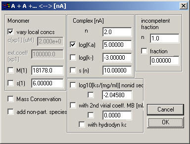
The only new input is n, the degree of association.
Again, note that the association constant is again the log10 of Ka in molar units. The default starting estimate shown here is Ka = 1x10(5)/Mn-1 . Except for at monomer-dimer association, if you have micromolar concentrations and see a significant fraction of oligomer, then this starting guess is probably much too low. If you estimate a concentration of equal monomer and n-mer to be at 10microM, then the log(Ka) value you should enter as starting guess is 5x(n-1).
The log(k-) entry describes for sedimentation velocity data the stability of the complex. The log(k-) is the base-10 log of the chemical off-rate constant of the n-mer. Values of > -1 (k- is faster than 0.1/sec) will switch the simulation to instantaneous equilibrium with mass action law fulfilled at all times and positions throughout the cell. Values smaller than -6 (koff < 1x10(-6)/sec) will lead to sedimentation profiles nearly identical to those of independently sedimenting populations of the free and complex species of the loading mixture.

The only difference between this and the previous model is that there are two association steps. The default is to describe them as monomer-dimer and monomer-tetramer. It is equivalent, however, to use monomer-dimer and dimer-tetramer associations. The latter can be an advantage since it's easier to make starting guesses. The disadvantage is that if you have a only little intermediate dimer but lots of tetramer, the dimerization could be very weak while tetramerization is very strong, which could be numerically inconvenient.
The log(k-2) entry describes for sedimentation velocity data the stability of the dimer (as base-10 log). Note that the off-rate constant for the tetramer is described as the base-10 log of the ratio of the off-rate constant of the tetramer (k-4) relative to that of the dimer (k-2).
If both off-rate constants are faster than 0.1/sec, this will switch the simulation to instantaneous equilibrium with mass action law fulfilled at all times and positions throughout the cell. Values smaller than -6 (koff < 1x10(-6)/sec) will lead to sedimentation profiles nearly identical to those of independently sedimenting populations of the free and complex species of the loading mixture.

Very analogous to the previous model.

Very similar, again, but you can freely specify the intermediate species (designated 'm') and the largest species ('n').