This model is for multi-component mixtures, and designed to take advantage of different extinction coefficient of the sedimenting protein components, in order to determine c(s) sedimentation coefficient distributions for each component in solution. This can enable to determine the composition of protein complexes, which can be highly useful in order to determine the association scheme and resolve multiple co-existing complexes.
In the simplest form, multiple signals are globally fitted as component sedimentation coefficient distributions
For stable mixtures on the time-scale of sedimentation, the interpretation is straight-forward, as the ck(s) distributions are simply molar sedimentation coefficient distributions of each component. This can be extended by applying constraints for minimal stoichiometries of larger species. For rapidly reversible interactions the complexes must be stabilized via mass action law, i.e. sufficiently high saturation of complexes in the reaction boundary must be maintained (e.g. loading concentrations > 5fold Kd).
A more detailed description of the theory and applications can be found in:
A. Balbo, K.H. Minor, C.A. Velikovsky, R.A. Mariuzza, C.B. Peterson, P. Schuck. Studying multi-protein complexes by multi-signal sedimentation velocity analytical ultracentrifugation. PNAS 102 (2005) 81-86
For the practical application in SedphaT, please familiarize yourself thoroughly with the hybrid discrete/continuous global c(s) model, as the multi-signal analysis is based on the same structure.
STEP 1: Planning of the Experiment
This analysis requires data acquisition at multiple signals. At least as many signals should be used as protein components are present. (Inclusion of a larger number of signals than of protein components is possible, and may have advantages.) Examples for possible configurations are:
* interference optical data + a single absorbance signal at either 230, 250, or 280 nm or VIS (for proteins), or 260 nm (nucleic acids)
* absorbance 280 nm + absorbance 250 nm
* absorbance 280 nm + absorbance 230 nm
* interference optical data + absorbance 280 nm + absorbance 250 nm
I found problematic the combination of absorbance 280, 250, and 230 due to the limited dynamic range of concentrations that can be observed, and also the use of far UV < 250 nm other than 230 nm (exploiting the UV lamp emission peak to improve the monochromaticity of the light).
Time required to scan multiple absorbance wavelengths is not a problem, and neither is the wavelength accuracy of the XLA/I as long as the wavelengths chosen are on a maximum or minimum of the extinction profile. Usually it is not necessary to drop the rotor speed in order to get a larger numbers of scans.
Obviously, the choice of the detection is dictated by the extinction coefficients of the components to be studied, which must be sufficiently different. Many proteins differ significantly in the signal increments of IF/UV280/UV250 due to different numbers of tryptophan and tyrosine residues, which can be used to distinguish them.
For the equivalent of the molar extinction coefficient for IF detection, use a value of of 3.3Mw/1.2, if Mw is the molar mass of the protein, and 1.2 cm is the pathlength of the cell. This is true, only, if there's no non-amino acid component in the protein: for example, glycosylation would change the IF signal increment of the protein.
For each protein component, the molar signal increment at one signal must be known. This can be either the IF signal increment, or (if the protein is modified) an extinction coefficient at a wavelength used in the data acquisition.
For discrimination of the protein components, the signal increments must be different at characteristic wavelengths. A simple test for unmodified proteins can be to calculate the weight-based extinction coefficient with SEDNTERP (OD/mg/ml), which should be >> 10% different for successful discrimination with IF/ABS280 signal combination. Alternatively, one can use SEDNTERP to plot the theoretical extinction spectrum, and estimate the ratio of extinction at 280 versus 250 nm. Again, two proteins can be distinguished by ABS280/ABS250 dual-wavelength detection if they differ in their extinction ratio.
Run each protein separately, in the same run with the the mixtures, in order to determine the extinction coefficients experimentally in the ultracentrifuge. See Step 3.
Load the data for each wavelength/signal separately as a new SV experiment.
When using multiple absorbance wavelength, it can be inconvenient to select the files of a certain wavelength only, because they are named by the XLA/I operating software in strict sequence of data acquisition, irrespective of wavelength. In this case, load all absorbance data and apply the SedfiT tool Save Raw Data Set (a function in the Loading Options) to write a copy of the absorbance files with altered filenames to the hard disk. The filenames will have information on the data acquisition wavelength (e.g. '50k280_001.ra2'), and this facilitates the selection of the velocity scans from each signal.
In my experience, a shift of wavelength by 1 or 2 nm is not detrimental to the data, and I would recommend loading all scans within a narrow range of wavelengths. As usual, load files from the beginning to the end of sedimentation, but avoid including a large number of scans that only show a completely depleted cell (this would slow down the calculations a lot).
You do not need to enter the extinction coefficients in the Experiment Parameter Box, as the extinction coefficients will be part of the global model. However, all other information, including meniscus, bottom, optical pathlength and links will be recognized and entered as usual. Usually, I consider TI noise components also for absorbance optical data.
In this way, create an xp file for each signal of each cell, and save each experiment to the hard disk with a characteristic name (e.g. 'ProteinA_cell1_IF.xp' and 'ProteinA_cell1_abs280.xp'). (Do not use empty spaces in any part of the data path or filename.)
After that, remove all experiments, and load only the xp-files corresponding to the different signals acquired for one cell. For example, load the IF and absorbance xp file of cell 1. The xp-files that belong to the same cell will constitute one 'SET'.
It is possible to load several SETS, for example, you could load the sequence cell1_IF.xp, cell1_ABS.xp, cell2_IF.xp, cell2_ABS.xp. Note that all files corresponding to the different signals included in a single SET have to be loaded in sequence, and that the sequence for all SETS has to be the same. When multiple SETS are loaded, in analogy to hybrid discrete/continuous model, global parameters to all SETS will be s and D, the frictional ratios, and the extinction coefficients. Local parameters will be the ck(s) distributions and concentrations. This will allow to utilize data from more than one cell in a global analysis. This can be used, for example, for a more precise determination of the extinction coefficients.
Consider linking meniscus and bottom for the multi-signal sets: Since the data are acquired from the same solution column, in principle the meniscus and bottom value should be the same. This is certainly true for different absorbance optical signals. It may not be true (and usually is not) between absorbance and interference optical data, due to the difficulty of a perfect radial calibration. Imperfect radial calibration of the IF system will create small offsets in the radius values, which (can usually be ignored in their effect on the measured s-value, but) require consideration of different apparent menisci positions for the IF and ABS data. This will create no further problem. After establishing links, make sure you update the xp-files with the function "Save All Experiments" (or control-A).
Next, go to the Model menu and click on 'multi-wavelength continuous/discrete distribution analysis'.
This will switch the multi-signal analysis on. A question will appear requesting the number of signals used in the analysis:
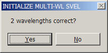
An algorithm is used to anticipate the number of signals - only two or three are currently implemented in SedphaT. (With commercial instruments, theoretically 4 signals can be acquired simultaneously, which may be included in the future.) It will be assumed that the experiments are in 'standard configuration', i.e. sequences of signals for each set are appended. If only one set is loaded (the example shown here), they are in 'standard configuration' by default.
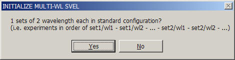
Note that the signal of the first xp-file will be designated wl1, the next one wl2 etc. This numbering scheme for the signals will be used in the following as a designation for referring to the different signals .
Save this state of SedphaT by saving current configuration to the hard disk. This way, everything done up to this point can be reproduced by double-clicking the corresponding .sedphat file.
STEP 3: Analysis of Extinction Coefficients
Make sure only the xp-files are loaded from the different signals of the cell containing one protein component alone, and that the multi-signal c(s) model is active. Click on Global Parameters. This will show the following parameter box:
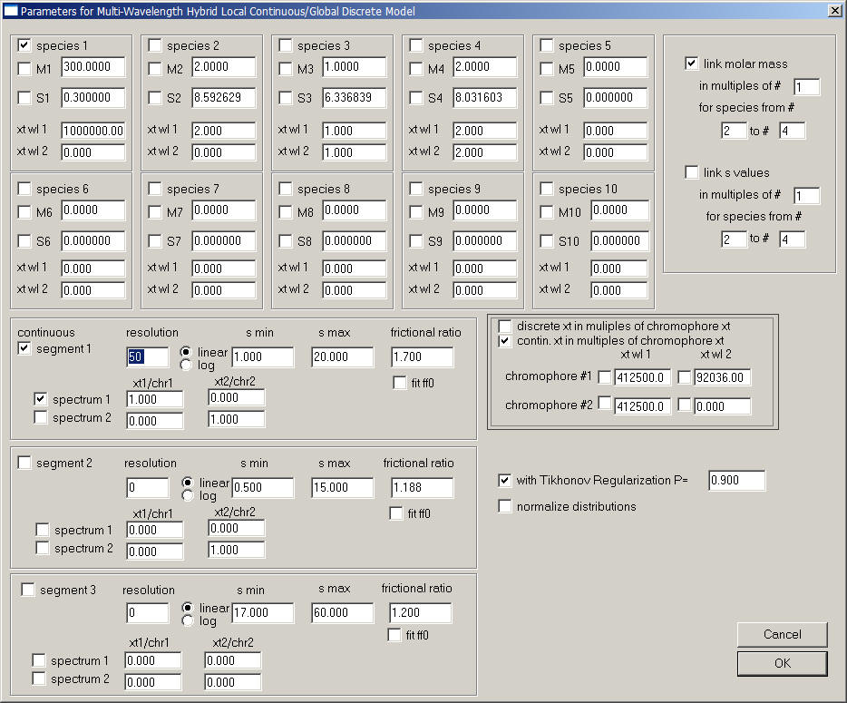
Note that most of the sections of this parameter box are very similar to those of the hybrid discrete/continous global c(s) model. Make sure you are familiar with those.
The different parts are:
1) the fields for the discrete species, for example species 1. s and M of the discrete species are treated as global parameters, while their concentration is local to each set.
Checking the box next to 'species 1' means it is utilized, unchecking takes it out of the fit. M and S fields are like in the hybrid discrete/continuous c(s) model. New are the fields "xt wl1" and "xt wl2", which are the molar signal increments (i.e. extinction coefficients) of this species for the signal designated "1" (the signal of the first xp file) and "2" (the signal of the second xp file).
2) The unit of the extinction coefficients to be entered depends on the state of the box in the new section:
This allows to define 'chromophors' or better 'chromophoric units' which are characterized by certain signal increments for both signals. For example, usually the chromophoric units will be the monomeric protein. The utility of the 'chromophor' is derived from the fact that it fixes the relative contributions to both signals, and that all possible species have signal contributions in multiples of these 'chromophoric units'.
For example, assume working with purified proteins that have different ratio of tryptophan and tyrosine, both proteins have a non-zero extinction coefficient at 280 nm, and data are acquired at 280 nm and in IF system. Assuming pure preparation, no species can occur that has signal contributions in the IF system only, and no species can have absorbance signal only. Further, the ratio of ABS280/IF signal cannot be lower than that of the protein with the smallest extinction coefficient at 280 nm. This requirement is a strong constraint for the analysis.
However, there can be exceptions. Consider that the IF data acquisition was superimposed by unmatched buffer salts. These obviously do not have UV signals. Therefore, it is possible to determine for the discrete species and the continuous distributions if their respective species extinction coefficients are expressed in multiples of chromophors, or not. In the case shown, the discrete species ARE NOT in multiples of chromophor extinction, while the continuous distributions ARE.
If you go back to species 1 above, you notice the effective M and s-values as they are usually observed for buffer salts. Signal 1 will be the IF signal, and the extinction coefficient entered is arbitrarily set to a value of 1000000, which will arbitrarily scale the signal of the buffer salt (we're not interested in this magnitude).
3) the sections for the segments of continuous distribution - There are up to three segments that can be used, and they are switched on with the check-mark in the upper left corner (e.g., next to 'segment 1'):
The parameters for the sedimentation coefficient distribution are like in the hybrid discrete/continuous global c(s) model.
New is the matrix for specifying the spectral properties of the c(s) components for this segment. For each segment, as many distributions can be calculated as there are different signal types. In the example for IF and ABS280 detection, that's two distributions. However, at this stage in the analysis we have data loaded from the cell with only a single component, and therefore there will only be one distribution needed. Therefore, the c(s) segment with component 'spectrum 1' is switched on, and the c(s) segment with component 'spectrum 2' is switched off.
For each c(s) component, we need to specify how the species will contribute to the different signals. This is what goes into these fields: for each c(s) component (row) we will enter the signal contribution to signal 1 (abbreviated here 'xt1') and signal 2 ('xt2'). This can be EITHER directly in the units of molar signal increments (i.e. molar extinction coefficients), OR in multiples of the chromophoric units ('chr1' and 'chr2') as defined above.
In this particular example, the unit of extinction coefficients is set for the continuous segments to be multiples of chromophores (see above). Therefore, the value '1.000' in the column of 'xt1/chr1' indicates the fact that all species in this component of this segment absorbs exactly like the chromophore 1. The value '0.000' in 'xt2/chr2' indicates that there is no contribution of the kind of chromophore 2 (there's only one protein in the solution considered so far).
4) Fitting the extinction coefficient: Notice that the definition of the chromophores and their signal increment includes check-marks for all fields.

These permit the signal increments to be treated as floating parameters. Although apparently all signal increments can be floated, at least one signal increment has to be known and remain constant (otherwise the signal increments will be completely correlated with the concentrations).
Since we only use a single chromophore in the analysis of this single protein component, only the first row of entries is used. In the following example, we have loaded the data such that the first xp file is IF data and the second is absorbance 280 nm data (abbreviated ABS280). Therefore, the first column will correspond to the interference signal increments. The protein considered in the example it an IgG, and with Mw = 150 kDa, we get 3.3x150000/1.2 = 412500 molar signal increment. The value of 100,000 is our starting estimate of the molar extinction coefficient at 280 nm, and the checkmark indicates that this will be floated in the analysis.
You can execute a run command to verify that no error message occurs. Also, different values for the extinction coefficient can be entered and the quality of fit compared. The fit is done best in two stages: a) switch OFF the meniscus and bottom variation for all xp files, and DO NOT float the f/f0 value of the continuous segment. In this way, only the discrete species and the extinction coefficient are non-linear unknowns, and the fit will converge rapidly to a very good value for the extinction coefficient; b) fine-tune by switching ON the meniscus and bottom variation for all xp files, as well as the f/f0 value of the continuous segment. Both parts work better with the Simplex algorithm (i.e. in the fitting options, switch Marquardt-Levenberg OFF).
My result is the following:

with xt280 = 206,740/Mcm . The green discrete species describes the buffer salt, and the red distribution all protein species with on average have a signal increment of 412,500/Mcm for IF and 206,740/Mcm in absorbance at 280 nm. In this determination we find that the main species is the IgG, but there are also substantial amount of aggregates and decay products. The information on the extinction coefficient is taken, conceptually, from the relative boundary heights in IF and absorbance detection.
One could wish for a determination of the extinction coefficients that excludes the decay products (< 6 S) and aggregates (> 9 S) from the determination of the IgG extinction coefficient. In this case, we set the fit up as following:

The discrete species is the IgG monomer, and now discrete species only are expressed in multiples of chromophore signal contributions. The continuous segments are specified directly in the form of molar extinction coefficients. Notice there are two continuous segments: segment 1 from 0.3 to 6 S for all species smaller than the IgG, and segment 2 for everything larger. Each segment has two separate component c(s), each one contributing only to one of the signals. This means that the two components now refer to IF and ABS280 signals only, which means that in this s-range the signal are essentially analyzed separately in conventional c(s) segments from analysis of the IF data, and from ABS280 data, respectively. The factor 100,000 is only introduced in order to scale the distributions. The result is shown here:
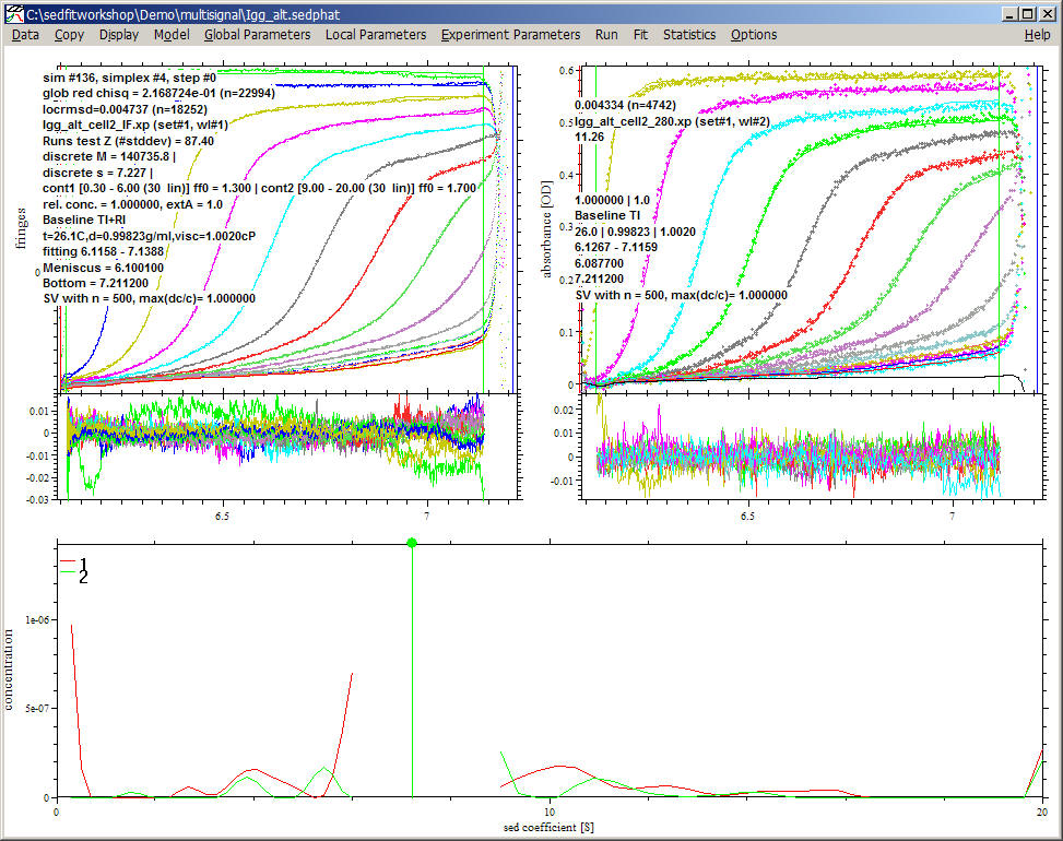
The red lines are the conventional c(s) segments from IF data (just scaled by 100,000) and the green lines those from absorbance data. Only the discrete species at 7.2 S is considered to contribute to both data sets, which results in an extinction coefficient at 280 nm of 210,754. This is only slightly different from the value obtained before, showing that the degradation products did not significantly bias the spectral analysis (most likely because they have very similar spectral properties).
This second, alternative analysis also spotlights another feature of the multi-signal analysis. Although not relevant for the determination of the IgG extinction coefficient, a close inspection of the c(s) segments for the IF and ABS data reveals a number of differences. The presence of a small species only contributing to IF signal was anticipated as the unmatched buffer salt. However, the 6S and 10 S species also only appear in the IF detection, while a 5.5 S peak is only visible in ABS detection. It is highly unlikely that such species really exist in solution, and they are a result of the insufficient information in the raw data on the precise s-values of these trace components. This will make their identification difficult. In contrast, in the multi-signal analysis above the IF and abs contributions of these trace components were constrained to the same ratio overall, with the result of a slightly worse but still acceptable fit, which utilizes both signals to arrive at a globally consistent picture.
STEP 4: Analysis of Component Sedimentation Coefficient Distributions
After the extinction coefficients are determined for each protein component, the mixture can be analyzed. The xp files from the different signals of the cell containing the mixture are loaded in the same way as described above.
In the following example, absorbance data at 280 nm are designated 'wl1' and IF data 'wl2', and we study a protein component with extinction coefficients 220,000 and 657,433/Mcm for ABS280 and IF, respectively, binding to a protein component with extinction coefficients 217,000 and 466,130/Mcm for ABS280 and IF, respecitvely. This can be specified as follows:

Note that there is only a single segment, consisting of two components. The spectrum of component 1 is identical to chromophore 1, and the spectrum of component 2 is identical to chromophore 2. Both are assumed to have the same frictional ratio.
Alternatively, they could have different frictional ratio if they were defined as two different segments with 1 component each, like this:

The global analysis gives two distributions, with the red line corresponding to component 1 and the green line to component 2, as indicated in the legend.

In this example, the protein designated component 1 consists of a monomer at 6 S and a dimer at 8 S, and very little higher s-value if studied by itself. Component 2 has a peak at 9 S if studied by itself, and some larger aggregates. Clearly, in the mixture here the protein 1 is co-sedimenting with protein 2, in approximately equimolar ratio for the peaks at 10 and 12 S.
The distributions can be integrated using the shortcut control-I, and zoomed in and out using the right mouse button. This is completely analogous to the integration and zoom functions for distributions in SEDFIT.
STEP 5: Application of Constraints for Stoichiometry
It is possible to apply additional constraints that reflect our hypothesis that all species > 10 S are complexes, which have stoichiometries of at least 1:1 or higher. For example, if we hypothesize from our knowledge of these proteins that there can only be species with molar ratios of 1:1, 1:2, up to 1:3, this can be expressed as follows:

The first segment up to 9S describes the free components only. Everything larger is considered a complex, described in segment 2. Here, there are two component distributions - one for the 1:1 stoichiometry of chromophoric units (i.e. 1:1 protein complex, since the chromophoric unit was taken as the protein spectrum), and one for a 1:3 stoichiometry of chromophoric units. If there was a 1:2 complex, it could not be distinguished from an equal amount of 1:1 and 1:3 stoichiometry.
More generally, these constraints are expressed as a change of the basis spectra as
(see PNAS 102 (2005) 81-86 for details).
In our example, the result shows four lines, two distributions from 0.5 to 9 S, and two from 9.5 to 25 S.
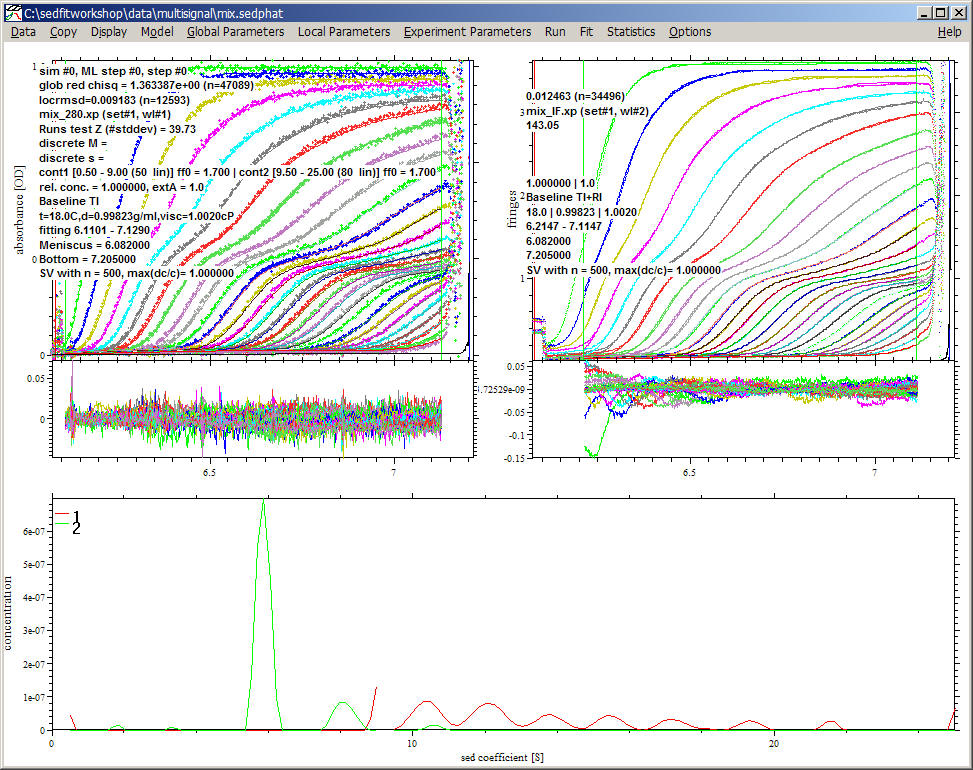
Note that the protein concentration is the area under the curve. The transition point for the first and second segment is 9S. Since this is just where the protein 1 had a peak before, the red line is now rising to a positive value at the maximum of 9S, and the area under the red curve from 8 - 9 S will approximately equal the area in the peak we saw before. Note that in this case, the appearance of a positive value of the distribution at the maximal s-value of the segment is not a problem, because larger sedimenting species are described in the fit. (They are just assumed to be complexes.) The second segment from 9.5 S to 25 S is almost exclusively populated by red species, which are the 1:1 complexes. Only a small trace of 1:3 complex at 10.5 S appears. Considering that the fit is virtually equally good as the one before, it can be said that the data is consistent with the hypothesis that all species > 10 S are a sequence of complexes, all with equimolar composition.
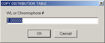
As in the hybrid discrete/continuous global c(s) model, one can retrieve the local concentrations of the discrete and the component c(s) segments via the copy command. If you copy the distribution, you will be asked:
1) for the discrete species

2) for each segment

and within each segment for each component:
etc., which will put the corresponding section of the hybrid distribution into the clipboard for pasting into your spreadsheet software.
Note that the component number when copying will not be the number specified in the parameter box, but they will be in sequence. For example, if component 1 was not utilized, and only component 2 was switched on, this will be copied by 'WL or Chromophore #' 1, instead of 2.