[ Up ] [ noninteracting discrete species ] [ self-association ] [ Nonideal Sedimentation ] [ c(M) ] [ c(M) with other prior ] [ c(s) ] [ c(s) with other prior ] [ c(s,M) and c(s,*) ] [ ls-g*(s) ] [ van Holde-Weischet ] [ ls-g*(s) with 1 discrete LE component ] [ extrapolate ls-g*(s) ] [ Analytical Zone Centrifugation ] [ DLS ] [ electrophoresis and other geometries ] [ Special ]

It can be useful to analyze data from dynamic light scattering in the same framework as the sedimentation velocity analysis.  Three models are available with SEDFIT:  that of superpositions of non-interacting species, hydrodynamic radius distributions, and diffusion coefficient distributions.  

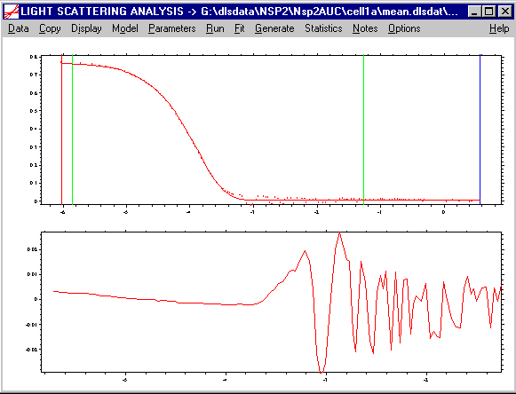
Currently, DLS data from Protein Solution and Brookhaven Instruments can be transformed into a Sedfit format, and then loaded into SEDFIT. After loading, they might look like this:

with a plot of the autocorrelation coefficients versus log₁₀(t) in the upper half, and the usual residuals plot in the lower.  Obviously, the entries for the meniscus and bottom are meaningless, but the position of the green lines still determines the range of the data to be analyzed.

All the models are based on the exponential expression for a single species field autocorrelation function.

(1)        

where t is the decay time and q=(4pn/l)sin(Q /2), with the solvent refractive index n, the wavelength of the incident light l, and the scattering angle Q.  Because the Lamm equation requires the diffusion coefficient, in principle, all Lamm equation models contain enough information to determine the autocorrelation functions.  

It should be noted that the scattering amplitude is proportional to the molar mass of the species, and the scattering intensity I replaces the concentration c.  

New 08/10/10: please see Jack Kornblatt's more detailed instructions for analyzing data from a Wyatt DynaPro Titan instrument.

New 08/10/10: more recently, models working directly with intensity autocorrelation functions are available, as well as cumulant analysis.

In this model, the diffusion coefficients are calculated in the same way as in the model for ideally sedimenting discrete species.  The same parameter input box is used.  Dependent on the setting of SEDFIT to use as fitting parameters (s,D) or (s,M) (see Fit M and s), the diffusion coefficient can either be directly determined or fitted, or the diffusion coefficient can be specified in terms of sedimentation coefficient and molar mass.  In this case, the Svedberg equation

(2)       

is used to calculate D, and it should be noted that the partial-specific volume and the buffer density needs to be properly adjusted. 

The analysis of DLS data in terms if molar mass and sedimentation coefficient can be advantageous if either the molar mass or the sedimentation coefficient is known.  

Great care should be taken to float only one parameter. Only either s, D, or M are determined by the data.  There is no check in SEDFIT for this, and correlated parameters may cause the program to crash.

These models are variants of the distribution analyses for sedimentation.  The light-scattering model is analogous to those presented in the introduction to size-distributions, but the kernel (i.e. the single-species model function) is adapted for DLS data analysis, by using Eq. 1 above.  In case of the diffusion coefficient distribution, D is directly used in the model for the autocorrelation function, in case of Rh-distribution, D is calculated via Stokes-Einstein equation.  All other parameters and distribution methods are similar to those for the continuous Lamm equation modeling, which makes this analysis very similar to the one performed in CONTIN described by Stephen Provencher (ref1).  Both the Tikhonov-Phillips and the maximum entropy regularization (default) can be used.  

The parameter box for the I(Rh) distribution looks like this: 

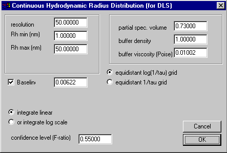
The meaning of the resolution, Rh min, Rh max and the confidence level is the same as in other distribution models.  It is useful to set the confidence level to a relatively small value (e.g. 0.55 ; but values below 0.5 are interpreted as no regularization).  The meaning of this parameter is strictly not a valid confidence level any more, because of the relatively small number of data points (compared to the resolution of the distribution).  [In the distribution calculations in SEDFIT, the degrees of freedom in the F-statistics are taken as equal to the number of data points, because of the large number of data points involved in sedimentation velocity data.  This approximation is not very good any more for small data sets such as DLS data when using the distribution model.]

When using the hydrodynamic radius distribution, of the field on the right-hand side only the viscosity is important, because the diffusion coefficients for each species is calculated using the Stokes-Einstein equation

(3)        

When using the diffusion coefficient distribution, none of the fields at the right-hand side is of any importance.

One difference to the c(s) and other distribution models is that here the Rh or D grid are spaced (and displayed) logarithmically, as this relates better to the resolution of the method.  However, one difficulty arises from the fact that the differential distribution functions can be either defined on a logarithmic scale, which displays the area under the curves in log units proportional to the scattering intensity of the subpopulations, or it can be defined in linear units, in which case the area under the curve does NOT correspond to the scattering intensity of the subpopulations.  However, in the latter case, if the data are (exported and) displayed on a linear scale, this relationship is restored.  [In short, this problem comes from the nonlinearity of the integration variable in log units.]  Therefore, which units are better depends on the framework of the desired interpretation.  For this reason, there is a switch in the parameter box allowing to change the integration variable between linear and log units.

A second switch is included for determining the spacing of the grid.  According to Livesey (ref 2), the best spacing of the grid when using maximum entropy regularization is equidistant on a log scale.  

The calculations are started with the Run command, and everything in the calculations is analogous to the other distribution models.  

A typical result is shown above.  Again, it should be noted that this the size-distribution here is in units of scattering intensity, not concentration.  

The DLS data result in significantly lower resolution than sedimentation velocity experiments, because of the smaller size-dependence of the diffusion coefficient (as compared to the sedimentation coefficients), and because of the ill-conditioned nature of the exponential functions (as opposed to the Lamm equation solutions). Nevertheless they can contribute very valuable complementary information to the study of complex mixtures of macromolecules.

References

(1) S.W. Provencher. (1982) A constrained regularization method for inverting data represented by linear algebraic or integral equations. Comp. Phys. Comm. 27:213-227

(2)  A.K. Livesey, P. Licinio, M. Delaye. (1986)  Maximum entropy analysis of quasielastic light scattering from colloidal dispersions. J. Chem. Phys. 84:5102-5107