continuous distribution c(M) Lamm equation model with other prior knowledge
with prior knowledge v-bar(M)
Model | continuous c(M) with prior knowledge | c(M) with prior knowledge v-bar(M)
This continuous distribution model is a special case of the c(M) distribution. The pages for size-distribution analysis, tutorial on size-distribution analysis, and on c(M) distribution should be consulted for more information.
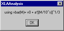
The only difference in the present model is the additional use prior knowledge on the partial-specific volume as a function of the molar mass of particles. When selecting this model, this is announced with a message box

indicating the use of the relationship

The parameters are entered in a series of input boxes, and the values are valid during the whole session with this model. They can be changed only by switching this model off, and reselecting it in the menu.
The first input is for a zero-order v-bar

followed by the amplitude a,

and the M-scale s on which this power-law applies.

The default values are those for floating lipid emulsion particles. After successful entry, a confirmation box appears.
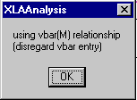
When using this model, the parameter input box (invoked by the parameter menu) is not different from that of the c(M) method. However, the v-bar entry in the parameter box can be ignored.
Model | continuous c(M) with prior knowledge | c(M) with invariant D
This continuous distribution model is another special case of the c(M) distribution. The pages for size-distribution analysis, tutorial on size-distribution analysis, and on c(M) distribution should be consulted for more information.
The central difference in the present model is that no assumption about the similarity of the shape is made. Sedimentation and diffusion coefficients are not calculated on the basis of a weight-average frictional ratio. Instead, knowledge is used directly about the diffusion coefficients. This can be useful if a sample is well-described by a single diffusion coefficient.
A single diffusion coefficient may be appropriate, for example, for samples that are not too heterogeneous, e.g. fractions from size-exclusion chromatography. Another example of using this model is the study of large particles with a small diffusion coefficient that is not strongly size-dependent, in experiments where sedimentation is rapid compared to diffusion. A third example are particles that have the same size (e.g. study of different iron-loading of ferritin).
This diffusion coefficient may be known from measurements by dynamic light scattering, or it can be fitted as an unknown.
Given the diffusion coefficient D, for each species the sedimentation coefficient s is calculated as a function of buoyant molar mass Mb
![]()
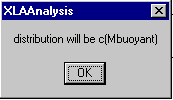
using the Svedberg relationship. For simplicity, the distribution will be calculated as buoyant molar mass distribution c(Mb). A reminder message box will appear.
A slightly modified input is required in the parameter box. No v-bar, buffer density, or viscosity is needed,
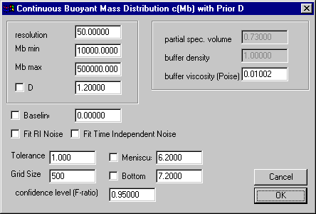
and the diffusion coefficient (in 10^-7 cm2/sec) will take the place of the f/f0 entry field. Everything else will work the same.