continuous distribution c(s) Lamm equation model with other prior knowledge
These models are very similar to the standard c(s) distribution. However, there are some differences in the prior knowledge. While the 'normal' c(s) distribution estimates the diffusion coefficients that belong to each s-value based on a weight-average frictional ratio, some additional or modified information can be entered in the following special cases:
Note: for a generalization of c(s) with other prior knowledge, look at the SedPHaT hybrid continuous/discrete model.
Continuous c(s) Conformational Change Model
The conformational change model allows to incorporate additional prior knowledge on one species with a known molar mass. This model is useful simply if one knows the molar mass of the main species. Because this species may undergo a conformational change, and therefore sediment with different s-values under different conditions, this model is suitable for such species with conformational change.
Essentially, this model assumes a constant molar mass for all species sedimenting in a specified range of s-values. Outside this range, a constant weight-average frictional ratio is assumed just like in the 'normal' c(s). The advantage of this model is an enhanced precision in the distribution analysis by making use of the known molar mass value, which allows to calculate a precise diffusion coefficient via the Svedberg equation for each s-value within the pre-defined range.
The parameters for this model look very much the same as in the normal c(s), except for the additional field in the top left corner, which contains the information on the single species with known molar mass:

The Mw field is for the molar mass (in Dalton, with buoyancy factor as specified in the v-bar and buffer density setting). The s-min and s-max directly under the Mw field determine the sedimentation coefficient range for which the molar mass value should be used. The meaning of all the other fields is exactly the same as in the normal c(s) model with constant frictional ratio.
In practice, it is probably necessary to run a normal c(s) first, in order to determine the s-range of the peak for the main species (or the one with the known molar mass, respectively). After that, this conformational change model can be used to produce a refined analysis.
New in version 8.5: There is the option to space the s-values logarithmically, which can be useful if a very large range of s-values has to be covered. Alternatively, a file containing a desired number and spacing of s-values can be read. The filename should be named 'sdist.ip1' (e.g., for scans series *.ip1) and be placed in the directory where the scans are located. Each time a distribution analysis is performed, such a file is automatically created, which can serve as a template for modification.
Continuous c(s) with constant D
The c(s) with constant D model is very similar to the normal c(s) model, but instead of using the approximation of similar shape (constant frictional ratio) for all molecules in the distribution, it uses the approximation of a constant diffusion coefficient.
This could be the approximately the case for narrow distributions, e.g. after fractionation by size-exclusion chromatography, or for molecules like ferritin, where the hydrodynamic radius of the molecules is constant throughout the distribution. An average D could be known from dynamic light scattering experiments, or the weight-average D can also be fitted to the data.
The parameter box looks very much like the one from c(s) analysis, but with two differences:

First, instead of the frictional ratio field we have now a field "D" for entering the diffusion coefficient (in 10-7 cm2/sec). As usual, if the check-box left to the D field is marked, this parameter will be fitted in a non-linear regression if the Fit command is used. The second difference is that the fields for the partial-specific volume, buffer density and viscosity are disabled, because they are not needed (these parameters were only used in the normal c(s) model to give us D from the combination of s and the frictional ratio).
New in version 8.5: There is the option to space the s-values logarithmically, which can be useful if a very large range of s-values has to be covered. Alternatively, a file containing a desired number and spacing of s-values can be read. The filename should be named 'sdist.ip1' (e.g., for scans series *.ip1) and be placed in the directory where the scans are located. Each time a distribution analysis is performed, such a file is automatically created, which can serve as a template for modification.
Continuous c(s) with 1 discrete component
This special case of the c(s) distribution analysis makes use of the knowledge of s and M for one particular molecule in solution. Imagine that we acquire interference optical data, but have more sodium chloride in the sample than in the reference solution. (Obviously, it would be better to do a dialysis, but this may not always be possible.) Such data may look like this:
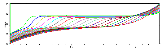
where clearly the sedimentation of a small component is superimposed to the macromolecular sedimentation. This model allows to include one additional discrete component that can take into account one such extra small molar mass component.
The parameter box looks like the normal c(s) parameters, but with two extra fields in the middle right: one for the sedimentation coefficient of the small component, and one for the molar mass (this refers to an 'effective' molar mass using the buoyancy as specified in the partial-specific volume and the buffer density field).
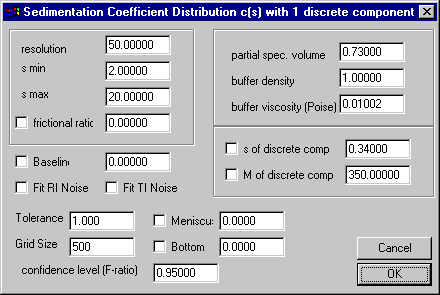
It is clear that allowing for the additional discrete small species will make the c(s) distribution dependent on the s and M of that species. In some situations, it may be possible to determine such an s and M value from independent experiments. More likely, however, the s and M of the discrete component has to be fitted by nonlinear regression (as usual, put a mark in the check-box to the left of the parameter and use the Fit command). This can be done similar to the optimization of the frictional ratio as shown in the tutorial, and should include as additional parameters to be optimized the meniscus and the bottom position of the solution column.
The resulting c(s) distribution of such a fit may look like this:
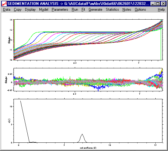
Please note the very large value at the first s-value - this is a result of the way the distribution is internally organized: The first data point of the c(s) distribution will be replaced by the discrete species. Therefore, export to a spreadsheet program (using the copy command, as described in the tutorial) is highly recommended for displaying the result. There, the first data point should be removed (or disregarded).
New in version 8.5: There is the option to space the s-values logarithmically, which can be useful if a very large range of s-values has to be covered. Alternatively, a file containing a desired number and spacing of s-values can be read. The filename should be named 'sdist.ip1' (e.g., for scans series *.ip1) and be placed in the directory where the scans are located. Each time a distribution analysis is performed, such a file is automatically created, which can serve as a template for modification.
Continuous c(s) with bi-modal f/f0
This special case of the c(s) distribution applies to systems where there are two clearly separated regions in the sedimentation coefficient distribution. In that case, it is usually possible to optimize two separate f/f0 parameters. The structure of the input box is similar as that for conformational change above: An area in the upper left corner specifies the f/f0 value for a particular region of the c(s) distribution. This f/f0 value can be fitted. Outside this special region, the distribution is calculated as usual using the frictional ratio in the middle section of the box.

Continuous c(s) with fix f/f0 and floating vbar
The idea of this model is that we may know relatively well the overall shape of a particle, but not its density. Imagine, for example, a protein-detergent complex where the detergent micelle is large compared to the protein, and/or where the protein is known not to be highly extended. In such a case, the frictional ratio may be close to unity (or the value for the detergent micelle alone, respectively). As a consequence, from the experimentally observed ratio of sedimentation relative to diffusion, the buoyancy factor can be extracted, i.e. the density increment (partial specific volume) of the protein-detergent complex.

Continuous c(s) for wormlike chain
This model is for flexible macromolecules that can be described as wormlike chains of subunits, where the subunits have known molar mass ('monomer Mw (Da)'), a known cross-section ('dehydrated cross-section (nm^2'), and an estimated hydration. It is envisioned to describe the sedimentation coefficient distributions of a mixture of long chains (much longer than monomer), which for a given molar mass distribution depends on the persistence length of the chains.
The persistence length can be either fixed or floated in the analysis. However, most likely for the envisioned application to long chains, the diffusion on the time-scale of sedimentation may be fairly small, such that the precision of the estimate of the persistence length from the fit may be relatively poor.

The mathematical formulas used are based on equations presented by Yamakawa-H and Fuji-M H [Yamakawa, M. Fujii (1973) Translational Friction coefficient of wormlike chains. Macromolecules 6 407-415] with the corrections given by Koenderink et al. [Gijsberta H. Koenderink, Karel L. Planken, Ramon Roozendaal,1, Albert P. Philipse (2005) Monodisperse DNA restriction fragments II. Sedimentation velocity and equilibrium experiments. Journal of Colloid and Interface Science 291 (2005) 126–134], implemented after code kindly provided by Christopher MacRaild and Geoffrey Howlett (see also MacRaild et al Biophys J. (2003) 2562-2569 ).
Continuous c(s) with M-s table
There are situations where we know a priori the relationship of the sedimentation coefficient as a function of molar mass. In this case, it is unnecessary and unproductive to make any assumptions. Instead, the known relationship can be used in SEDFIT. (Knowing s and M, obviously allows to calculate D, which will be used in the Lamm equation solution for the particular s-value.)
To do this, you need to create a file "mofs.dat" in the folder "c:\sedfit". This file may be created, for example, with the notepad. It must contain two columns, where the first is the s-value (s20w in S), the second is the molar mass (kDa) that belongs to this s-value. It may look like this:
1 1
2 5
3 20
4 50
5 80
6 100
7 150
8 180
9 200
10 250
15 400
20 800
25 1500
Note, there's no need to have any specific spacing (except the s-values must be monotonically increasing). SEDFIT will use linear interpolation to derive Mw-values for intermediate s-values as appropriate.

Important: The s-values are in s20w! SEDFIT will assume that the v-bar, buffer density and viscosity have been set properly in this box. The final output will be the usual experimental s-value scale. Only for using the lookup table, internally a conversion to s20w is made. But for consistency with the other models, the output is done in experimental s-values.